Phylogenetics with Bio.Phylo
The Bio.Phylo module was introduced in Biopython 1.54. Following the lead of SeqIO and AlignIO, it aims to provide a common way to work with phylogenetic trees independently of the source data format, as well as a consistent API for I/O operations.
Bio.Phylo is described in an open-access journal article Talevich et al. 2012 [Talevich2012], which you might also find helpful.
Demo: What’s in a Tree?
To get acquainted with the module, let’s start with a tree that we’ve already constructed, and inspect it a few different ways. Then we’ll colorize the branches, to use a special phyloXML feature, and finally save it.
Create a simple Newick file named simple.dnd using your favorite
text editor, or use
simple.dnd
provided with the Biopython source code:
(((A,B),(C,D)),(E,F,G));
This tree has no branch lengths, only a topology and labeled terminals. (If you have a real tree file available, you can follow this demo using that instead.)
Launch the Python interpreter of your choice:
$ ipython -pylab
For interactive work, launching the IPython interpreter with the
-pylab flag enables matplotlib integration, so graphics will pop
up automatically. We’ll use that during this demo.
Now, within Python, read the tree file, giving the file name and the name of the format.
>>> from Bio import Phylo
>>> tree = Phylo.read("simple.dnd", "newick")
Printing the tree object as a string gives us a look at the entire object hierarchy.
>>> print(tree)
Tree(rooted=False, weight=1.0)
    Clade()
        Clade()
            Clade()
                Clade(name='A')
                Clade(name='B')
            Clade()
                Clade(name='C')
                Clade(name='D')
        Clade()
            Clade(name='E')
            Clade(name='F')
            Clade(name='G')
The Tree object contains global information about the tree, such as
whether it’s rooted or unrooted. It has one root clade, and under that,
it’s nested lists of clades all the way down to the tips.
The function draw_ascii creates a simple ASCII-art (plain text)
dendrogram. This is a convenient visualization for interactive
exploration, in case better graphical tools aren’t available.
>>> from Bio import Phylo
>>> tree = Phylo.read("simple.dnd", "newick")
>>> Phylo.draw_ascii(tree)
                                                    ________________________ A
                           ________________________|
                          |                        |________________________ B
  ________________________|
 |                        |                         ________________________ C
 |                        |________________________|
_|                                                 |________________________ D
 |
 |                         ________________________ E
 |                        |
 |________________________|________________________ F
                          |
                          |________________________ G
If you have matplotlib or pylab installed, you can create a
graphical tree using the draw function.
>>> tree.rooted = True
>>> Phylo.draw(tree)
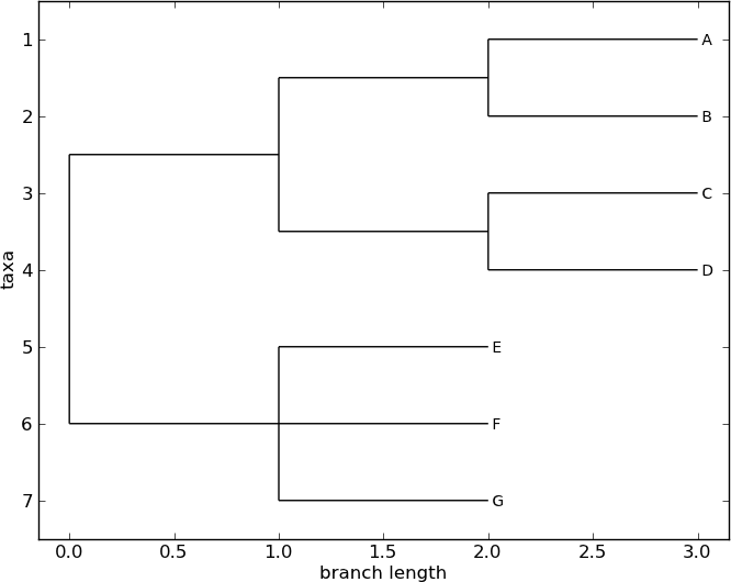
Fig. 6 A rooted tree drawn with Phylo.draw.
See Fig. 6.
Coloring branches within a tree
The function draw supports the display of different colors and
branch widths in a tree. As of Biopython 1.59, the color and
width attributes are available on the basic Clade object and there’s
nothing extra required to use them. Both attributes refer to the branch
leading the given clade, and apply recursively, so all descendent
branches will also inherit the assigned width and color values during
display.
In earlier versions of Biopython, these were special features of PhyloXML trees, and using the attributes required first converting the tree to a subclass of the basic tree object called Phylogeny, from the Bio.Phylo.PhyloXML module.
In Biopython 1.55 and later, this is a convenient tree method:
>>> tree = tree.as_phyloxml()
In Biopython 1.54, you can accomplish the same thing with one extra import:
>>> from Bio.Phylo.PhyloXML import Phylogeny
>>> tree = Phylogeny.from_tree(tree)
Note that the file formats Newick and Nexus don’t support branch colors or widths, so if you use these attributes in Bio.Phylo, you will only be able to save the values in PhyloXML format. (You can still save a tree as Newick or Nexus, but the color and width values will be skipped in the output file.)
Now we can begin assigning colors. First, we’ll color the root clade gray. We can do that by assigning the 24-bit color value as an RGB triple, an HTML-style hex string, or the name of one of the predefined colors.
>>> tree.root.color = (128, 128, 128)
Or:
>>> tree.root.color = "#808080"
Or:
>>> tree.root.color = "gray"
Colors for a clade are treated as cascading down through the entire clade, so when we colorize the root here, it turns the whole tree gray. We can override that by assigning a different color lower down on the tree.
Let’s target the most recent common ancestor (MRCA) of the nodes named
“E” and “F”. The common_ancestor method returns a reference to that
clade in the original tree, so when we color that clade “salmon”, the
color will show up in the original tree.
>>> mrca = tree.common_ancestor({"name": "E"}, {"name": "F"})
>>> mrca.color = "salmon"
If we happened to know exactly where a certain clade is in the tree, in
terms of nested list entries, we can jump directly to that position in
the tree by indexing it. Here, the index [0,1] refers to the second
child of the first child of the root.
>>> tree.clade[0, 1].color = "blue"
Finally, show our work:
>>> Phylo.draw(tree)
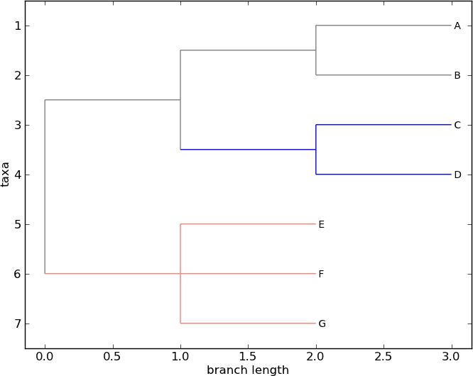
Fig. 7 A colorized tree drawn with Phylo.draw.
See Fig. 7.
Note that a clade’s color includes the branch leading to that clade, as well as its descendents. The common ancestor of E and F turns out to be just under the root, and with this coloring we can see exactly where the root of the tree is.
Drawing trees with iplotx
For users seeking advanced styling options, Bio.Phylo trees are natively
supported by the external library iplotx:
https://iplotx.readthedocs.io/en/latest/
iplotx enables customisation of many aspects of the visualisation,
including layout, vertex and branch properties, cascading backgrounds,
and labels. Here is a self-contained example.
>>> from Bio import Phylo
>>> import iplotx as ipx
>>> tree = Phylo.read("simple.dnd", "newick")
>>> ipx.tree(tree, leaf_deep=True, leaf_labels=True, style="tree")
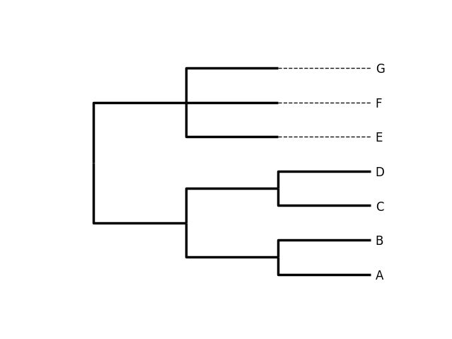
iplotx has an extensive gallery of examples.
Writing tree to file
My, we’ve accomplished a lot! Let’s take a break here and save our work.
Call the write function with a file name or handle — here we use
standard output, to see what would be written — and the format
phyloxml. PhyloXML saves the colors we assigned, so you can open
this phyloXML file in another tree viewer like Archaeopteryx, and the
colors will show up there, too.
>>> import sys
>>> n = Phylo.write(tree, sys.stdout, "phyloxml")
<phyloxml ...>
  <phylogeny rooted="true">
    <clade>
      <color>
        <red>128</red>
        <green>128</green>
        <blue>128</blue>
      </color>
      <clade>
        <clade>
          <clade>
            <name>A</name>
          </clade>
          <clade>
            <name>B</name>
          </clade>
        </clade>
        <clade>
          <color>
            <red>0</red>
            <green>0</green>
            <blue>255</blue>
          </color>
          <clade>
            <name>C</name>
          </clade>
          ...
    </clade>
  </phylogeny>
</phyloxml>
>>> n
1
The rest of this chapter covers the core functionality of Bio.Phylo in greater detail. For more examples of using Bio.Phylo, see the cookbook page on Biopython.org:
I/O functions
Like SeqIO and AlignIO, Phylo handles file input and output through four
functions: parse, read, write and convert, all of which
support the tree file formats Newick, NEXUS, phyloXML and NeXML, as well
as the Comparative Data Analysis Ontology (CDAO).
The read function parses a single tree in the given file and returns
it. Careful; it will raise an error if the file contains more than one
tree, or no trees.
>>> from Bio import Phylo
>>> tree = Phylo.read("Tests/Nexus/int_node_labels.nwk", "newick")
>>> print(tree)
Tree(rooted=False, weight=1.0)
    Clade(branch_length=75.0, name='gymnosperm')
        Clade(branch_length=25.0, name='Coniferales')
            Clade(branch_length=25.0)
                Clade(branch_length=10.0, name='Tax+nonSci')
                    Clade(branch_length=90.0, name='Taxaceae')
                        Clade(branch_length=125.0, name='Cephalotaxus')
                        ...
(Example files are available in the Tests/Nexus/ and
Tests/PhyloXML/ directories of the Biopython distribution.)
To handle multiple (or an unknown number of) trees, use the parse
function iterates through each of the trees in the given file:
>>> trees = Phylo.parse("Tests/PhyloXML/phyloxml_examples.xml", "phyloxml")
>>> for tree in trees:
...     print(tree)
...
Phylogeny(description='phyloXML allows to use either a "branch_length" attribute...', name='example from Prof. Joe Felsenstein's book "Inferring Phyl...', rooted=True)
    Clade()
        Clade(branch_length=0.06)
            Clade(branch_length=0.102, name='A')
            ...
Write a tree or iterable of trees back to file with the write
function:
>>> trees = Phylo.parse("Tests/PhyloXML/phyloxml_examples.xml", "phyloxml")
>>> tree1 = next(trees)
>>> Phylo.write(tree1, "tree1.nwk", "newick")
1
>>> Phylo.write(trees, "other_trees.xml", "phyloxml")  # write the remaining trees
13
Convert files between any of the supported formats with the convert
function:
>>> Phylo.convert("tree1.nwk", "newick", "tree1.xml", "nexml")
1
>>> Phylo.convert("other_trees.xml", "phyloxml", "other_trees.nex", "nexus")
13
To use strings as input or output instead of actual files, use
StringIO as you would with SeqIO and AlignIO:
>>> from Bio import Phylo
>>> from io import StringIO
>>> handle = StringIO("(((A,B),(C,D)),(E,F,G));")
>>> tree = Phylo.read(handle, "newick")
View and export trees
The simplest way to get an overview of a Tree object is to print
it:
>>> from Bio import Phylo
>>> tree = Phylo.read("PhyloXML/example.xml", "phyloxml")
>>> print(tree)
Phylogeny(description='phyloXML allows to use either a "branch_length" attribute...', name='example from Prof. Joe Felsenstein's book "Inferring Phyl...', rooted=True)
    Clade()
        Clade(branch_length=0.06)
            Clade(branch_length=0.102, name='A')
            Clade(branch_length=0.23, name='B')
        Clade(branch_length=0.4, name='C')
This is essentially an outline of the object hierarchy Biopython uses to represent a tree. But more likely, you’d want to see a drawing of the tree. There are three functions to do this.
As we saw in the demo, draw_ascii prints an ascii-art drawing of the
tree (a rooted phylogram) to standard output, or an open file handle if
given. Not all of the available information about the tree is shown, but
it provides a way to quickly view the tree without relying on any
external dependencies.
>>> tree = Phylo.read("PhyloXML/example.xml", "phyloxml")
>>> Phylo.draw_ascii(tree)
             __________________ A
  __________|
_|          |___________________________________________ B
 |
 |___________________________________________________________________________ C
The draw function draws a more attractive image using the matplotlib
library. See the API documentation for details on the arguments it
accepts to customize the output.
>>> Phylo.draw(tree, branch_labels=lambda c: c.branch_length)
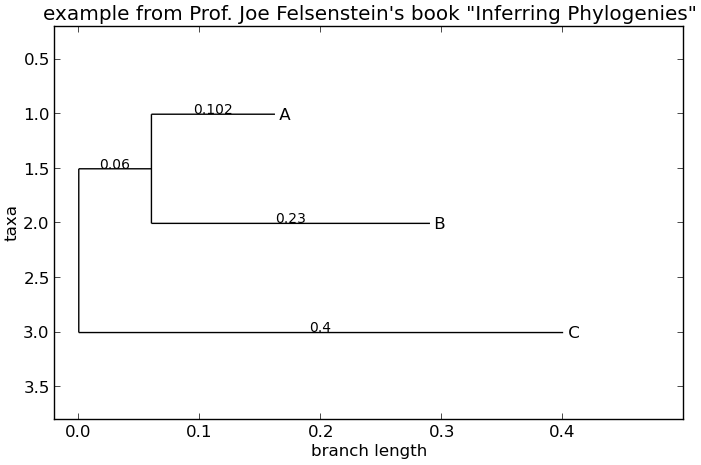
Fig. 8 A simple rooted tree plotted with the draw function.
See Fig. 8 for example.
See the Phylo page on the Biopython wiki
(http://biopython.org/wiki/Phylo) for descriptions and examples of the
more advanced functionality in draw_ascii, draw_graphviz and
to_networkx.
Using Tree and Clade objects
The Tree objects produced by parse and read are containers
for recursive sub-trees, attached to the Tree object at the root
attribute (whether or not the phylogenetic tree is actually considered
rooted). A Tree has globally applied information for the phylogeny,
such as rootedness, and a reference to a single Clade; a Clade
has node- and clade-specific information, such as branch length, and a
list of its own descendent Clade instances, attached at the
clades attribute.
So there is a distinction between tree and tree.root. In
practice, though, you rarely need to worry about it. To smooth over the
difference, both Tree and Clade inherit from TreeMixin,
which contains the implementations for methods that would be commonly
used to search, inspect or modify a tree or any of its clades. This
means that almost all of the methods supported by tree are also
available on tree.root and any clade below it. (Clade also has a
root property, which returns the clade object itself.)
Search and traversal methods
For convenience, we provide a couple of simplified methods that return all external or internal nodes directly as a list:
get_terminalsmakes a list of all of this tree’s terminal (leaf) nodes.
get_nonterminalsmakes a list of all of this tree’s nonterminal (internal) nodes.
These both wrap a method with full control over tree traversal,
find_clades. Two more traversal methods, find_elements and
find_any, rely on the same core functionality and accept the same
arguments, which we’ll call a “target specification” for lack of a
better description. These specify which objects in the tree will be
matched and returned during iteration. The first argument can be any of
the following types:
A TreeElement instance, which tree elements will match by identity — so searching with a Clade instance as the target will find that clade in the tree;
A string, which matches tree elements’ string representation — in particular, a clade’s
name(added in Biopython 1.56);A class or type, where every tree element of the same type (or sub-type) will be matched;
A dictionary where keys are tree element attributes and values are matched to the corresponding attribute of each tree element. This one gets even more elaborate:
If an
intis given, it matches numerically equal attributes, e.g. 1 will match 1 or 1.0If a boolean is given (True or False), the corresponding attribute value is evaluated as a boolean and checked for the same
NonematchesNoneIf a string is given, the value is treated as a regular expression (which must match the whole string in the corresponding element attribute, not just a prefix). A given string without special regex characters will match string attributes exactly, so if you don’t use regexes, don’t worry about it. For example, in a tree with clade names Foo1, Foo2 and Foo3,
tree.find_clades({"name": "Foo1"})matches Foo1,{"name": "Foo.*"}matches all three clades, and{"name": "Foo"}doesn’t match anything.
Since floating-point arithmetic can produce some strange behavior, we don’t support matching
floats directly. Instead, use the booleanTrueto match every element with a nonzero value in the specified attribute, then filter on that attribute manually with an inequality (or exact number, if you like living dangerously).If the dictionary contains multiple entries, a matching element must match each of the given attribute values — think “and”, not “or”.
A function taking a single argument (it will be applied to each element in the tree), returning True or False. For convenience, LookupError, AttributeError and ValueError are silenced, so this provides another safe way to search for floating-point values in the tree, or some more complex characteristic.
After the target, there are two optional keyword arguments:
- terminal
— A boolean value to select for or against terminal clades (a.k.a. leaf nodes): True searches for only terminal clades, False for non-terminal (internal) clades, and the default, None, searches both terminal and non-terminal clades, as well as any tree elements lacking the
is_terminalmethod.- order
— Tree traversal order:
"preorder"(default) is depth-first search,"postorder"is DFS with child nodes preceding parents, and"level"is breadth-first search.
Finally, the methods accept arbitrary keyword arguments which are
treated the same way as a dictionary target specification: keys indicate
the name of the element attribute to search for, and the argument value
(string, integer, None or boolean) is compared to the value of each
attribute found. If no keyword arguments are given, then any TreeElement
types are matched. The code for this is generally shorter than passing a
dictionary as the target specification:
tree.find_clades({"name": "Foo1"}) can be shortened to
tree.find_clades(name="Foo1").
(In Biopython 1.56 or later, this can be even shorter:
tree.find_clades("Foo1"))
Now that we’ve mastered target specifications, here are the methods used to traverse a tree:
find_cladesFind each clade containing a matching element. That is, find each element as with
find_elements, but return the corresponding clade object. (This is usually what you want.)The result is an iterable through all matching objects, searching depth-first by default. This is not necessarily the same order as the elements appear in the Newick, Nexus or XML source file!
find_elementsFind all tree elements matching the given attributes, and return the matching elements themselves. Simple Newick trees don’t have complex sub-elements, so this behaves the same as
find_cladeson them. PhyloXML trees often do have complex objects attached to clades, so this method is useful for extracting those.find_anyReturn the first element found by
find_elements(), or None. This is also useful for checking whether any matching element exists in the tree, and can be used in a conditional.
Two more methods help navigating between nodes in the tree:
get_pathList the clades directly between the tree root (or current clade) and the given target. Returns a list of all clade objects along this path, ending with the given target, but excluding the root clade.
traceList of all clade object between two targets in this tree. Excluding start, including finish.
Information methods
These methods provide information about the whole tree (or any clade).
common_ancestorFind the most recent common ancestor of all the given targets. (This will be a Clade object). If no target is given, returns the root of the current clade (the one this method is called from); if 1 target is given, this returns the target itself. However, if any of the specified targets are not found in the current tree (or clade), an exception is raised.
count_terminalsCounts the number of terminal (leaf) nodes within the tree.
depthsCreate a mapping of tree clades to depths. The result is a dictionary where the keys are all of the Clade instances in the tree, and the values are the distance from the root to each clade (including terminals). By default the distance is the cumulative branch length leading to the clade, but with the
unit_branch_lengths=Trueoption, only the number of branches (levels in the tree) is counted.distanceCalculate the sum of the branch lengths between two targets. If only one target is specified, the other is the root of this tree.
total_branch_lengthCalculate the sum of all the branch lengths in this tree. This is usually just called the “length” of the tree in phylogenetics, but we use a more explicit name to avoid confusion with Python terminology.
The rest of these methods are boolean checks:
is_bifurcatingTrue if the tree is strictly bifurcating; i.e. all nodes have either 2 or 0 children (internal or external, respectively). The root may have 3 descendents and still be considered part of a bifurcating tree.
is_monophyleticTest if all of the given targets comprise a complete subclade — i.e., there exists a clade such that its terminals are the same set as the given targets. The targets should be terminals of the tree. For convenience, this method returns the common ancestor (MCRA) of the targets if they are monophyletic (instead of the value
True), andFalseotherwise.is_parent_ofTrue if target is a descendent of this tree — not required to be a direct descendent. To check direct descendents of a clade, simply use list membership testing:
if subclade in clade: ...is_preterminalTrue if all direct descendents are terminal; False if any direct descendent is not terminal.
Modification methods
These methods modify the tree in-place. If you want to keep the original
tree intact, make a complete copy of the tree first, using Python’s
copy module:
tree = Phylo.read("example.xml", "phyloxml")
import copy

newtree = copy.deepcopy(tree)
collapseDeletes the target from the tree, relinking its children to its parent.
collapse_allCollapse all the descendents of this tree, leaving only terminals. Branch lengths are preserved, i.e. the distance to each terminal stays the same. With a target specification (see above), collapses only the internal nodes matching the specification.
ladderizeSort clades in-place according to the number of terminal nodes. Deepest clades are placed last by default. Use
reverse=Trueto sort clades deepest-to-shallowest.prunePrunes a terminal clade from the tree. If the taxon is from a bifurcation, the connecting node will be collapsed and its branch length added to remaining terminal node. This might no longer be a meaningful value.
root_with_outgroupReroot this tree with the outgroup clade containing the given targets, i.e. the common ancestor of the outgroup. This method is only available on Tree objects, not Clades.
If the outgroup is identical to self.root, no change occurs. If the outgroup clade is terminal (e.g. a single terminal node is given as the outgroup), a new bifurcating root clade is created with a 0-length branch to the given outgroup. Otherwise, the internal node at the base of the outgroup becomes a trifurcating root for the whole tree. If the original root was bifurcating, it is dropped from the tree.
In all cases, the total branch length of the tree stays the same.
root_at_midpointReroot this tree at the calculated midpoint between the two most distant tips of the tree. (This uses
root_with_outgroupunder the hood.)splitGenerate n (default 2) new descendants. In a species tree, this is a speciation event. New clades have the given
branch_lengthand the same name as this clade’s root plus an integer suffix (counting from 0) — for example, splitting a clade named “A” produces the sub-clades “A0” and “A1”.
See the Phylo page on the Biopython wiki (http://biopython.org/wiki/Phylo) for more examples of using the available methods.
Features of PhyloXML trees
The phyloXML file format includes fields for annotating trees with additional data types and visual cues.
See the PhyloXML page on the Biopython wiki (http://biopython.org/wiki/PhyloXML) for descriptions and examples of using the additional annotation features provided by PhyloXML.
Running external applications
While Bio.Phylo doesn’t infer trees from alignments itself, there are
third-party programs available that do. These can be accessed from
within python by using the subprocess module.
Below is an example on how to use a python script to interact with PhyML
(http://www.atgc-montpellier.fr/phyml/). The program accepts an input
alignment in phylip-relaxed format (that’s Phylip format, but
without the 10-character limit on taxon names) and a variety of options.
>>> import subprocess
>>> cmd = "phyml -i Tests/Phylip/random.phy"
>>> results = subprocess.run(cmd, shell=True, stdout=subprocess.PIPE, text=True)
The ‘stdout = subprocess.PIPE‘ argument makes the output of the program accessible through ‘results.stdout‘ for debugging purposes, (the same can be done for ‘stderr‘), and ‘text=True‘ makes the returned information be a python string, instead of a ‘bytes‘ object.
This generates a tree file and a stats file with the names
[input filename]_phyml_tree.txt and
[input filename]_phyml_stats.txt. The tree file is in Newick
format:
>>> from Bio import Phylo
>>> tree = Phylo.read("Tests/Phylip/random.phy_phyml_tree.txt", "newick")
>>> Phylo.draw_ascii(tree)
  __________________ F
 |
 | I
 |
_|                     ________ C
 |            ________|
 |           |        |        , J
 |           |        |________|
 |           |                 |          , H
 |___________|                 |__________|
             |                            |______________ D
             |
             , G
             |
             |                , E
             |________________|
                              |                 ___________________________ A
                              |________________|
                                               |_________ B
The subprocess module can also be used for interacting with any
other programs that provide a command line interface such as RAxML
(https://sco.h-its.org/exelixis/software.html), FastTree
(http://www.microbesonline.org/fasttree/), dnaml and protml.
PAML integration
Biopython 1.58 brought support for PAML (http://abacus.gene.ucl.ac.uk/software/paml.html), a suite of programs for phylogenetic analysis by maximum likelihood. Currently the programs codeml, baseml and yn00 are implemented. Due to PAML’s usage of control files rather than command line arguments to control runtime options, usage of this wrapper strays from the format of other application wrappers in Biopython.
A typical workflow would be to initialize a PAML object, specifying an
alignment file, a tree file, an output file and a working directory.
Next, runtime options are set via the set_options() method or by
reading an existing control file. Finally, the program is run via the
run() method and the output file is automatically parsed to a
results dictionary.
Here is an example of typical usage of codeml:
>>> from Bio.Phylo.PAML import codeml
>>> cml = codeml.Codeml()
>>> cml.alignment = "Tests/PAML/Alignments/alignment.phylip"
>>> cml.tree = "Tests/PAML/Trees/species.tree"
>>> cml.out_file = "results.out"
>>> cml.working_dir = "./scratch"
>>> cml.set_options(
...     seqtype=1,
...     verbose=0,
...     noisy=0,
...     RateAncestor=0,
...     model=0,
...     NSsites=[0, 1, 2],
...     CodonFreq=2,
...     cleandata=1,
...     fix_alpha=1,
...     kappa=4.54006,
... )
>>> results = cml.run()
>>> ns_sites = results.get("NSsites")
>>> m0 = ns_sites.get(0)
>>> m0_params = m0.get("parameters")
>>> print(m0_params.get("omega"))
Existing output files may be parsed as well using a module’s read()
function:
>>> results = codeml.read("Tests/PAML/Results/codeml/codeml_NSsites_all.out")
>>> print(results.get("lnL max"))
Detailed documentation for this new module currently lives on the Biopython wiki: http://biopython.org/wiki/PAML
Future plans
Bio.Phylo is under active development. Here are some features we might add in future releases:
- New methods
Generally useful functions for operating on Tree or Clade objects appear on the Biopython wiki first, so that casual users can test them and decide if they’re useful before we add them to Bio.Phylo:
- Bio.Nexus port
Much of this module was written during Google Summer of Code 2009, under the auspices of NESCent, as a project to implement Python support for the phyloXML data format (see Features of PhyloXML trees). Support for Newick and Nexus formats was added by porting part of the existing Bio.Nexus module to the new classes used by Bio.Phylo.
Currently, Bio.Nexus contains some useful features that have not yet been ported to Bio.Phylo classes — notably, calculating a consensus tree. If you find some functionality lacking in Bio.Phylo, try poking through Bio.Nexus to see if it’s there instead.
We’re open to any suggestions for improving the functionality and usability of this module; just let us know on the mailing list or our bug database.
Finally, if you need additional functionality not yet included in the Phylo module, check if it’s available in another of the high-quality Python libraries for phylogenetics such as DendroPy (https://dendropy.org/) or PyCogent (http://pycogent.org/). Since these libraries also support standard file formats for phylogenetic trees, you can easily transfer data between libraries by writing to a temporary file or StringIO object.