Cookbook – Cool things to do with it

Biopython now has two collections of “cookbook” examples – this chapter (which has been included in this tutorial for many years and has gradually grown), and http://biopython.org/wiki/Category:Cookbook which is a user contributed collection on our wiki.

We’re trying to encourage Biopython users to contribute their own examples to the wiki. In addition to helping the community, one direct benefit of sharing an example like this is that you could also get some feedback on the code from other Biopython users and developers - which could help you improve all your Python code.

In the long term, we may end up moving all of the examples in this chapter to the wiki, or elsewhere within the tutorial.

Working with sequence files

This section shows some more examples of sequence input/output, using the Bio.SeqIO module described in Chapter Sequence Input/Output.

Filtering a sequence file

Often you’ll have a large file with many sequences in it (e.g. FASTA file or genes, or a FASTQ or SFF file of reads), a separate shorter list of the IDs for a subset of sequences of interest, and want to make a new sequence file for this subset.

Let’s say the list of IDs is in a simple text file, as the first word on each line. This could be a tabular file where the first column is the ID. Try something like this:

from Bio import SeqIO

input_file = "big_file.sff"
id_file = "short_list.txt"
output_file = "short_list.sff"

with open(id_file) as id_handle:
    wanted = set(line.rstrip("\n").split(None, 1)[0] for line in id_handle)
print("Found %i unique identifiers in %s" % (len(wanted), id_file))

records = (r for r in SeqIO.parse(input_file, "sff") if r.id in wanted)
count = SeqIO.write(records, output_file, "sff")
print("Saved %i records from %s to %s" % (count, input_file, output_file))
if count < len(wanted):
    print("Warning %i IDs not found in %s" % (len(wanted) - count, input_file))

Note that we use a Python set rather than a list, this makes testing membership faster.

As discussed in Section Low level FASTA and FASTQ parsers, for a large FASTA or FASTQ file for speed you would be better off not using the high-level SeqIO interface, but working directly with strings. This next example shows how to do this with FASTQ files – it is more complicated:

from Bio.SeqIO.QualityIO import FastqGeneralIterator

input_file = "big_file.fastq"
id_file = "short_list.txt"
output_file = "short_list.fastq"

with open(id_file) as id_handle:
    # Taking first word on each line as an identifier
    wanted = set(line.rstrip("\n").split(None, 1)[0] for line in id_handle)
print("Found %i unique identifiers in %s" % (len(wanted), id_file))

with open(input_file) as in_handle:
    with open(output_file, "w") as out_handle:
        for title, seq, qual in FastqGeneralIterator(in_handle):
            # The ID is the first word in the title line (after the @ sign):
            if title.split(None, 1)[0] in wanted:
                # This produces a standard 4-line FASTQ entry:
                out_handle.write("@%s\n%s\n+\n%s\n" % (title, seq, qual))
                count += 1
print("Saved %i records from %s to %s" % (count, input_file, output_file))
if count < len(wanted):
    print("Warning %i IDs not found in %s" % (len(wanted) - count, input_file))

Producing randomized genomes

Let’s suppose you are looking at genome sequence, hunting for some sequence feature – maybe extreme local GC% bias, or possible restriction digest sites. Once you’ve got your Python code working on the real genome it may be sensible to try running the same search on randomized versions of the same genome for statistical analysis (after all, any “features” you’ve found could just be there just by chance).

For this discussion, we’ll use the GenBank file for the pPCP1 plasmid from Yersinia pestis biovar Microtus. The file is included with the Biopython unit tests under the GenBank folder, or you can get it from our website, `NC_005816.gb <https://raw.githubusercontent.com/biopython/biopython/master/Tests/GenBank/NC_005816.gb>`__. This file contains one and only one record, so we can read it in as a SeqRecord using the Bio.SeqIO.read() function:

>>> from Bio import SeqIO
>>> original_rec = SeqIO.read("NC_005816.gb", "genbank")

So, how can we generate a shuffled versions of the original sequence? I would use the built in Python random module for this, in particular the function random.shuffle – but this works on a Python list. Our sequence is a Seq object, so in order to shuffle it we need to turn it into a list:

>>> import random
>>> nuc_list = list(original_rec.seq)
>>> random.shuffle(nuc_list)  # acts in situ!

Now, in order to use Bio.SeqIO to output the shuffled sequence, we need to construct a new SeqRecord with a new Seq object using this shuffled list. In order to do this, we need to turn the list of nucleotides (single letter strings) into a long string – the standard Python way to do this is with the string object’s join method.

>>> from Bio.Seq import Seq
>>> from Bio.SeqRecord import SeqRecord
>>> shuffled_rec = SeqRecord(
...     Seq("".join(nuc_list)), id="Shuffled", description="Based on %s" % original_rec.id
... )

Let’s put all these pieces together to make a complete Python script which generates a single FASTA file containing 30 randomly shuffled versions of the original sequence.

This first version just uses a big for loop and writes out the records one by one (using the SeqRecord’s format method described in Section Getting your SeqRecord objects as formatted strings):

import random
from Bio.Seq import Seq
from Bio.SeqRecord import SeqRecord
from Bio import SeqIO

original_rec = SeqIO.read("NC_005816.gb", "genbank")

with open("shuffled.fasta", "w") as output_handle:
    for i in range(30):
        nuc_list = list(original_rec.seq)
        random.shuffle(nuc_list)
        shuffled_rec = SeqRecord(
            Seq("".join(nuc_list)),
            id="Shuffled%i" % (i + 1),
            description="Based on %s" % original_rec.id,
        )
        output_handle.write(shuffled_rec.format("fasta"))

Personally I prefer the following version using a function to shuffle the record and a generator expression instead of the for loop:

import random
from Bio.Seq import Seq
from Bio.SeqRecord import SeqRecord
from Bio import SeqIO


def make_shuffle_record(record, new_id):
    nuc_list = list(record.seq)
    random.shuffle(nuc_list)
    return SeqRecord(
        Seq("".join(nuc_list)),
        id=new_id,
        description="Based on %s" % original_rec.id,
    )


original_rec = SeqIO.read("NC_005816.gb", "genbank")
shuffled_recs = (
    make_shuffle_record(original_rec, "Shuffled%i" % (i + 1)) for i in range(30)
)

SeqIO.write(shuffled_recs, "shuffled.fasta", "fasta")

Translating a FASTA file of CDS entries

Suppose you’ve got an input file of CDS entries for some organism, and you want to generate a new FASTA file containing their protein sequences. i.e. Take each nucleotide sequence from the original file, and translate it. Back in Section Translation we saw how to use the Seq object’s translate method, and the optional cds argument which enables correct translation of alternative start codons.

We can combine this with Bio.SeqIO as shown in the reverse complement example in Section Converting a file of sequences to their reverse complements. The key point is that for each nucleotide SeqRecord, we need to create a protein SeqRecord - and take care of naming it.

You can write you own function to do this, choosing suitable protein identifiers for your sequences, and the appropriate genetic code. In this example we just use the default table and add a prefix to the identifier:

from Bio.SeqRecord import SeqRecord


def make_protein_record(nuc_record):
    """Returns a new SeqRecord with the translated sequence (default table)."""
    return SeqRecord(
        seq=nuc_record.seq.translate(cds=True),
        id="trans_" + nuc_record.id,
        description="translation of CDS, using default table",
    )

We can then use this function to turn the input nucleotide records into protein records ready for output. An elegant way and memory efficient way to do this is with a generator expression:

from Bio import SeqIO

proteins = (
    make_protein_record(nuc_rec)
    for nuc_rec in SeqIO.parse("coding_sequences.fasta", "fasta")
)
SeqIO.write(proteins, "translations.fasta", "fasta")

This should work on any FASTA file of complete coding sequences. If you are working on partial coding sequences, you may prefer to use nuc_record.seq.translate(to_stop=True) in the example above, as this wouldn’t check for a valid start codon etc.

Making the sequences in a FASTA file upper case

Often you’ll get data from collaborators as FASTA files, and sometimes the sequences can be in a mixture of upper and lower case. In some cases this is deliberate (e.g. lower case for poor quality regions), but usually it is not important. You may want to edit the file to make everything consistent (e.g. all upper case), and you can do this easily using the upper() method of the SeqRecord object (added in Biopython 1.55):

from Bio import SeqIO

records = (rec.upper() for rec in SeqIO.parse("mixed.fas", "fasta"))
count = SeqIO.write(records, "upper.fas", "fasta")
print("Converted %i records to upper case" % count)

How does this work? The first line is just importing the Bio.SeqIO module. The second line is the interesting bit – this is a Python generator expression which gives an upper case version of each record parsed from the input file (mixed.fas). In the third line we give this generator expression to the Bio.SeqIO.write() function and it saves the new upper cases records to our output file (upper.fas).

The reason we use a generator expression (rather than a list or list comprehension) is this means only one record is kept in memory at a time. This can be really important if you are dealing with large files with millions of entries.

Sorting a sequence file

Suppose you wanted to sort a sequence file by length (e.g. a set of contigs from an assembly), and you are working with a file format like FASTA or FASTQ which Bio.SeqIO can read, write (and index).

If the file is small enough, you can load it all into memory at once as a list of SeqRecord objects, sort the list, and save it:

from Bio import SeqIO

records = list(SeqIO.parse("ls_orchid.fasta", "fasta"))
records.sort(key=lambda r: len(r))
SeqIO.write(records, "sorted_orchids.fasta", "fasta")

The only clever bit is specifying a comparison method for how to sort the records (here we sort them by length). If you wanted the longest records first, you could flip the comparison or use the reverse argument:

from Bio import SeqIO

records = list(SeqIO.parse("ls_orchid.fasta", "fasta"))
records.sort(key=lambda r: -len(r))
SeqIO.write(records, "sorted_orchids.fasta", "fasta")

Now that’s pretty straight forward - but what happens if you have a very large file and you can’t load it all into memory like this? For example, you might have some next-generation sequencing reads to sort by length. This can be solved using the Bio.SeqIO.index() function.

from Bio import SeqIO

# Get the lengths and ids, and sort on length
len_and_ids = sorted(
    (len(rec), rec.id) for rec in SeqIO.parse("ls_orchid.fasta", "fasta")
)
ids = reversed([id for (length, id) in len_and_ids])
del len_and_ids  # free this memory
record_index = SeqIO.index("ls_orchid.fasta", "fasta")
records = (record_index[id] for id in ids)
SeqIO.write(records, "sorted.fasta", "fasta")

First we scan through the file once using Bio.SeqIO.parse(), recording the record identifiers and their lengths in a list of tuples. We then sort this list to get them in length order, and discard the lengths. Using this sorted list of identifiers Bio.SeqIO.index() allows us to retrieve the records one by one, and we pass them to Bio.SeqIO.write() for output.

These examples all use Bio.SeqIO to parse the records into SeqRecord objects which are output using Bio.SeqIO.write(). What if you want to sort a file format which Bio.SeqIO.write() doesn’t support, like the plain text SwissProt format? Here is an alternative solution using the get_raw() method added to Bio.SeqIO.index() in Biopython 1.54 (see Section Getting the raw data for a record).

from Bio import SeqIO

# Get the lengths and ids, and sort on length
len_and_ids = sorted(
    (len(rec), rec.id) for rec in SeqIO.parse("ls_orchid.fasta", "fasta")
)
ids = reversed([id for (length, id) in len_and_ids])
del len_and_ids  # free this memory

record_index = SeqIO.index("ls_orchid.fasta", "fasta")
with open("sorted.fasta", "wb") as out_handle:
    for id in ids:
        out_handle.write(record_index.get_raw(id))

Note with Python 3 onwards, we have to open the file for writing in binary mode because the get_raw() method returns bytes objects.

As a bonus, because it doesn’t parse the data into SeqRecord objects a second time it should be faster. If you only want to use this with FASTA format, we can speed this up one step further by using the low-level FASTA parser to get the record identifiers and lengths:

from Bio.SeqIO.FastaIO import SimpleFastaParser
from Bio import SeqIO

# Get the lengths and ids, and sort on length
with open("ls_orchid.fasta") as in_handle:
    len_and_ids = sorted(
        (len(seq), title.split(None, 1)[0])
        for title, seq in SimpleFastaParser(in_handle)
    )
ids = reversed([id for (length, id) in len_and_ids])
del len_and_ids  # free this memory

record_index = SeqIO.index("ls_orchid.fasta", "fasta")
with open("sorted.fasta", "wb") as out_handle:
    for id in ids:
        out_handle.write(record_index.get_raw(id))

Simple quality filtering for FASTQ files

The FASTQ file format was introduced at Sanger and is now widely used for holding nucleotide sequencing reads together with their quality scores. FASTQ files (and the related QUAL files) are an excellent example of per-letter-annotation, because for each nucleotide in the sequence there is an associated quality score. Any per-letter-annotation is held in a SeqRecord in the letter_annotations dictionary as a list, tuple or string (with the same number of elements as the sequence length).

One common task is taking a large set of sequencing reads and filtering them (or cropping them) based on their quality scores. The following example is very simplistic, but should illustrate the basics of working with quality data in a SeqRecord object. All we are going to do here is read in a file of FASTQ data, and filter it to pick out only those records whose PHRED quality scores are all above some threshold (here 20).

For this example we’ll use some real data downloaded from the ENA sequence read archive, ftp://ftp.sra.ebi.ac.uk/vol1/fastq/SRR020/SRR020192/SRR020192.fastq.gz (2MB) which unzips to a 19MB file SRR020192.fastq. This is some Roche 454 GS FLX single end data from virus infected California sea lions (see https://www.ebi.ac.uk/ena/data/view/SRS004476 for details).

First, let’s count the reads:

from Bio import SeqIO

count = 0
for rec in SeqIO.parse("SRR020192.fastq", "fastq"):
    count += 1
print("%i reads" % count)

Now let’s do a simple filtering for a minimum PHRED quality of 20:

from Bio import SeqIO

good_reads = (
    rec
    for rec in SeqIO.parse("SRR020192.fastq", "fastq")
    if min(rec.letter_annotations["phred_quality"]) >= 20
)
count = SeqIO.write(good_reads, "good_quality.fastq", "fastq")
print("Saved %i reads" % count)

This pulled out only \(14580\) reads out of the \(41892\) present. A more sensible thing to do would be to quality trim the reads, but this is intended as an example only.

FASTQ files can contain millions of entries, so it is best to avoid loading them all into memory at once. This example uses a generator expression, which means only one SeqRecord is created at a time - avoiding any memory limitations.

Note that it would be faster to use the low-level FastqGeneralIterator parser here (see Section Low level FASTA and FASTQ parsers), but that does not turn the quality string into integer scores.

Trimming off primer sequences

For this example we’re going to pretend that GATGACGGTGT is a 5’ primer sequence we want to look for in some FASTQ formatted read data. As in the example above, we’ll use the SRR020192.fastq file downloaded from the ENA (ftp://ftp.sra.ebi.ac.uk/vol1/fastq/SRR020/SRR020192/SRR020192.fastq.gz).

By using the main Bio.SeqIO interface, the same approach would work with any other supported file format (e.g. FASTA files). However, for large FASTQ files it would be faster the low-level FastqGeneralIterator parser here (see the earlier example, and Section Low level FASTA and FASTQ parsers).

This code uses Bio.SeqIO with a generator expression (to avoid loading all the sequences into memory at once), and the Seq object’s startswith method to see if the read starts with the primer sequence:

from Bio import SeqIO

primer_reads = (
    rec
    for rec in SeqIO.parse("SRR020192.fastq", "fastq")
    if rec.seq.startswith("GATGACGGTGT")
)
count = SeqIO.write(primer_reads, "with_primer.fastq", "fastq")
print("Saved %i reads" % count)

That should find \(13819\) reads from SRR014849.fastq and save them to a new FASTQ file, with_primer.fastq.

Now suppose that instead you wanted to make a FASTQ file containing these reads but with the primer sequence removed? That’s just a small change as we can slice the SeqRecord (see Section Slicing a SeqRecord) to remove the first eleven letters (the length of our primer):

from Bio import SeqIO

trimmed_primer_reads = (
    rec[11:]
    for rec in SeqIO.parse("SRR020192.fastq", "fastq")
    if rec.seq.startswith("GATGACGGTGT")
)
count = SeqIO.write(trimmed_primer_reads, "with_primer_trimmed.fastq", "fastq")
print("Saved %i reads" % count)

Again, that should pull out the \(13819\) reads from SRR020192.fastq, but this time strip off the first ten characters, and save them to another new FASTQ file, with_primer_trimmed.fastq.

Now, suppose you want to create a new FASTQ file where these reads have their primer removed, but all the other reads are kept as they were? If we want to still use a generator expression, it is probably clearest to define our own trim function:

from Bio import SeqIO


def trim_primer(record, primer):
    if record.seq.startswith(primer):
        return record[len(primer) :]
    else:
        return record


trimmed_reads = (
    trim_primer(record, "GATGACGGTGT")
    for record in SeqIO.parse("SRR020192.fastq", "fastq")
)
count = SeqIO.write(trimmed_reads, "trimmed.fastq", "fastq")
print("Saved %i reads" % count)

This takes longer, as this time the output file contains all \(41892\) reads. Again, we’re used a generator expression to avoid any memory problems. You could alternatively use a generator function rather than a generator expression.

from Bio import SeqIO


def trim_primers(records, primer):
    """Removes perfect primer sequences at start of reads.

    This is a generator function, the records argument should
    be a list or iterator returning SeqRecord objects.
    """
    len_primer = len(primer)  # cache this for later
    for record in records:
        if record.seq.startswith(primer):
            yield record[len_primer:]
        else:
            yield record


original_reads = SeqIO.parse("SRR020192.fastq", "fastq")
trimmed_reads = trim_primers(original_reads, "GATGACGGTGT")
count = SeqIO.write(trimmed_reads, "trimmed.fastq", "fastq")
print("Saved %i reads" % count)

This form is more flexible if you want to do something more complicated where only some of the records are retained – as shown in the next example.

Trimming off adaptor sequences

This is essentially a simple extension to the previous example. We are going to going to pretend GATGACGGTGT is an adaptor sequence in some FASTQ formatted read data, again the SRR020192.fastq file from the NCBI (ftp://ftp.sra.ebi.ac.uk/vol1/fastq/SRR020/SRR020192/SRR020192.fastq.gz).

This time however, we will look for the sequence anywhere in the reads, not just at the very beginning:

from Bio import SeqIO


def trim_adaptors(records, adaptor):
    """Trims perfect adaptor sequences.

    This is a generator function, the records argument should
    be a list or iterator returning SeqRecord objects.
    """
    len_adaptor = len(adaptor)  # cache this for later
    for record in records:
        index = record.seq.find(adaptor)
        if index == -1:
            # adaptor not found, so won't trim
            yield record
        else:
            # trim off the adaptor
            yield record[index + len_adaptor :]


original_reads = SeqIO.parse("SRR020192.fastq", "fastq")
trimmed_reads = trim_adaptors(original_reads, "GATGACGGTGT")
count = SeqIO.write(trimmed_reads, "trimmed.fastq", "fastq")
print("Saved %i reads" % count)

Because we are using a FASTQ input file in this example, the SeqRecord objects have per-letter-annotation for the quality scores. By slicing the SeqRecord object the appropriate scores are used on the trimmed records, so we can output them as a FASTQ file too.

Compared to the output of the previous example where we only looked for a primer/adaptor at the start of each read, you may find some of the trimmed reads are quite short after trimming (e.g. if the adaptor was found in the middle rather than near the start). So, let’s add a minimum length requirement as well:

from Bio import SeqIO


def trim_adaptors(records, adaptor, min_len):
    """Trims perfect adaptor sequences, checks read length.

    This is a generator function, the records argument should
    be a list or iterator returning SeqRecord objects.
    """
    len_adaptor = len(adaptor)  # cache this for later
    for record in records:
        len_record = len(record)  # cache this for later
        if len(record) < min_len:
            # Too short to keep
            continue
        index = record.seq.find(adaptor)
        if index == -1:
            # adaptor not found, so won't trim
            yield record
        elif len_record - index - len_adaptor >= min_len:
            # after trimming this will still be long enough
            yield record[index + len_adaptor :]


original_reads = SeqIO.parse("SRR020192.fastq", "fastq")
trimmed_reads = trim_adaptors(original_reads, "GATGACGGTGT", 100)
count = SeqIO.write(trimmed_reads, "trimmed.fastq", "fastq")
print("Saved %i reads" % count)

By changing the format names, you could apply this to FASTA files instead. This code also could be extended to do a fuzzy match instead of an exact match (maybe using a pairwise alignment, or taking into account the read quality scores), but that will be much slower.

Converting FASTQ files

Back in Section Converting between sequence file formats we showed how to use Bio.SeqIO to convert between two file formats. Here we’ll go into a little more detail regarding FASTQ files which are used in second generation DNA sequencing. Please refer to Cock et al. (2010) [Cock2010] for a longer description. FASTQ files store both the DNA sequence (as a string) and the associated read qualities.

PHRED scores (used in most FASTQ files, and also in QUAL files, ACE files and SFF files) have become a de facto standard for representing the probability of a sequencing error (here denoted by \(P_e\)) at a given base using a simple base ten log transformation:

\[Q_{\textrm{PHRED}} = - 10 \times \textrm{log}_{10} ( P_e )\]

This means a wrong read (\(P_e = 1\)) gets a PHRED quality of \(0\), while a very good read like \(P_e = 0.00001\) gets a PHRED quality of \(50\). While for raw sequencing data qualities higher than this are rare, with post processing such as read mapping or assembly, qualities of up to about \(90\) are possible (indeed, the MAQ tool allows for PHRED scores in the range 0 to 93 inclusive).

The FASTQ format has the potential to become a de facto standard for storing the letters and quality scores for a sequencing read in a single plain text file. The only fly in the ointment is that there are at least three versions of the FASTQ format which are incompatible and difficult to distinguish…

1. The original Sanger FASTQ format uses PHRED qualities encoded with an ASCII offset of 33. The NCBI are using this format in their Short Read Archive. We call this the fastq (or fastq-sanger) format in Bio.SeqIO.

2. Solexa (later bought by Illumina) introduced their own version using Solexa qualities encoded with an ASCII offset of 64. We call this the fastq-solexa format.

3. Illumina pipeline 1.3 onwards produces FASTQ files with PHRED qualities (which is more consistent), but encoded with an ASCII offset of 64. We call this the fastq-illumina format.

The Solexa quality scores are defined using a different log transformation:

\[Q_{\textrm{Solexa}} = - 10 \times \textrm{log}_{10} \left( \frac{P_e}{1-P_e} \right)\]

Given Solexa/Illumina have now moved to using PHRED scores in version 1.3 of their pipeline, the Solexa quality scores will gradually fall out of use. If you equate the error estimates (\(P_e\)) these two equations allow conversion between the two scoring systems - and Biopython includes functions to do this in the Bio.SeqIO.QualityIO module, which are called if you use Bio.SeqIO to convert an old Solexa/Illumina file into a standard Sanger FASTQ file:

from Bio import SeqIO

SeqIO.convert("solexa.fastq", "fastq-solexa", "standard.fastq", "fastq")

If you want to convert a new Illumina 1.3+ FASTQ file, all that gets changed is the ASCII offset because although encoded differently the scores are all PHRED qualities:

from Bio import SeqIO

SeqIO.convert("illumina.fastq", "fastq-illumina", "standard.fastq", "fastq")

Note that using Bio.SeqIO.convert() like this is much faster than combining Bio.SeqIO.parse() and Bio.SeqIO.write() because optimized code is used for converting between FASTQ variants (and also for FASTQ to FASTA conversion).

For good quality reads, PHRED and Solexa scores are approximately equal, which means since both the fasta-solexa and fastq-illumina formats use an ASCII offset of 64 the files are almost the same. This was a deliberate design choice by Illumina, meaning applications expecting the old fasta-solexa style files will probably be OK using the newer fastq-illumina files (on good data). Of course, both variants are very different from the original FASTQ standard as used by Sanger, the NCBI, and elsewhere (format name fastq or fastq-sanger).

For more details, see the built in help (also online):

>>> from Bio.SeqIO import QualityIO
>>> help(QualityIO)

Converting FASTA and QUAL files into FASTQ files

FASTQ files hold both sequences and their quality strings. FASTA files hold just sequences, while QUAL files hold just the qualities. Therefore a single FASTQ file can be converted to or from paired FASTA and QUAL files.

Going from FASTQ to FASTA is easy:

from Bio import SeqIO

SeqIO.convert("example.fastq", "fastq", "example.fasta", "fasta")

Going from FASTQ to QUAL is also easy:

from Bio import SeqIO

SeqIO.convert("example.fastq", "fastq", "example.qual", "qual")

However, the reverse is a little more tricky. You can use Bio.SeqIO.parse() to iterate over the records in a single file, but in this case we have two input files. There are several strategies possible, but assuming that the two files are really paired the most memory efficient way is to loop over both together. The code is a little fiddly, so we provide a function called PairedFastaQualIterator in the Bio.SeqIO.QualityIO module to do this. This takes two handles (the FASTA file and the QUAL file) and returns a SeqRecord iterator:

from Bio.SeqIO.QualityIO import PairedFastaQualIterator

for record in PairedFastaQualIterator(open("example.fasta"), open("example.qual")):
    print(record)

This function will check that the FASTA and QUAL files are consistent (e.g. the records are in the same order, and have the same sequence length). You can combine this with the Bio.SeqIO.write() function to convert a pair of FASTA and QUAL files into a single FASTQ files:

from Bio import SeqIO
from Bio.SeqIO.QualityIO import PairedFastaQualIterator

with open("example.fasta") as f_handle, open("example.qual") as q_handle:
    records = PairedFastaQualIterator(f_handle, q_handle)
    count = SeqIO.write(records, "temp.fastq", "fastq")
print("Converted %i records" % count)

Indexing a FASTQ file

FASTQ files are usually very large, with millions of reads in them. Due to the sheer amount of data, you can’t load all the records into memory at once. This is why the examples above (filtering and trimming) iterate over the file looking at just one SeqRecord at a time.

However, sometimes you can’t use a big loop or an iterator - you may need random access to the reads. Here the Bio.SeqIO.index() function may prove very helpful, as it allows you to access any read in the FASTQ file by its name (see Section Sequence files as Dictionaries – Indexed files).

Again we’ll use the SRR020192.fastq file from the ENA (ftp://ftp.sra.ebi.ac.uk/vol1/fastq/SRR020/SRR020192/SRR020192.fastq.gz), although this is actually quite a small FASTQ file with less than \(50,000\) reads:

>>> from Bio import SeqIO
>>> fq_dict = SeqIO.index("SRR020192.fastq", "fastq")
>>> len(fq_dict)
41892
>>> list(fq_dict.keys())[:4]
['SRR020192.38240', 'SRR020192.23181', 'SRR020192.40568', 'SRR020192.23186']
>>> fq_dict["SRR020192.23186"].seq
Seq('GTCCCAGTATTCGGATTTGTCTGCCAAAACAATGAAATTGACACAGTTTACAAC...CCG')

When testing this on a FASTQ file with seven million reads, indexing took about a minute, but record access was almost instant.

The sister function Bio.SeqIO.index_db() lets you save the index to an SQLite3 database file for near instantaneous reuse - see Section Sequence files as Dictionaries – Indexed files for more details.

The example in Section Sorting a sequence file show how you can use the Bio.SeqIO.index() function to sort a large FASTA file – this could also be used on FASTQ files.

Converting SFF files

If you work with 454 (Roche) sequence data, you will probably have access to the raw data as a Standard Flowgram Format (SFF) file. This contains the sequence reads (called bases) with quality scores and the original flow information.

A common task is to convert from SFF to a pair of FASTA and QUAL files, or to a single FASTQ file. These operations are trivial using the Bio.SeqIO.convert() function (see Section Converting between sequence file formats):

>>> from Bio import SeqIO
>>> SeqIO.convert("E3MFGYR02_random_10_reads.sff", "sff", "reads.fasta", "fasta")
10
>>> SeqIO.convert("E3MFGYR02_random_10_reads.sff", "sff", "reads.qual", "qual")
10
>>> SeqIO.convert("E3MFGYR02_random_10_reads.sff", "sff", "reads.fastq", "fastq")
10

Remember the convert function returns the number of records, in this example just ten. This will give you the untrimmed reads, where the leading and trailing poor quality sequence or adaptor will be in lower case. If you want the trimmed reads (using the clipping information recorded within the SFF file) use this:

>>> from Bio import SeqIO
>>> SeqIO.convert("E3MFGYR02_random_10_reads.sff", "sff-trim", "trimmed.fasta", "fasta")
10
>>> SeqIO.convert("E3MFGYR02_random_10_reads.sff", "sff-trim", "trimmed.qual", "qual")
10
>>> SeqIO.convert("E3MFGYR02_random_10_reads.sff", "sff-trim", "trimmed.fastq", "fastq")
10

If you run Linux, you could ask Roche for a copy of their “off instrument” tools (often referred to as the Newbler tools). This offers an alternative way to do SFF to FASTA or QUAL conversion at the command line (but currently FASTQ output is not supported), e.g.

$ sffinfo -seq -notrim E3MFGYR02_random_10_reads.sff > reads.fasta
$ sffinfo -qual -notrim E3MFGYR02_random_10_reads.sff > reads.qual
$ sffinfo -seq -trim E3MFGYR02_random_10_reads.sff > trimmed.fasta
$ sffinfo -qual -trim E3MFGYR02_random_10_reads.sff > trimmed.qual

The way Biopython uses mixed case sequence strings to represent the trimming points deliberately mimics what the Roche tools do.

For more information on the Biopython SFF support, consult the built in help:

>>> from Bio.SeqIO import SffIO
>>> help(SffIO)

Identifying open reading frames

A very simplistic first step at identifying possible genes is to look for open reading frames (ORFs). By this we mean look in all six frames for long regions without stop codons – an ORF is just a region of nucleotides with no in frame stop codons.

Of course, to find a gene you would also need to worry about locating a start codon, possible promoters – and in Eukaryotes there are introns to worry about too. However, this approach is still useful in viruses and Prokaryotes.

To show how you might approach this with Biopython, we’ll need a sequence to search, and as an example we’ll again use the bacterial plasmid – although this time we’ll start with a plain FASTA file with no pre-marked genes: `NC_005816.fna <https://raw.githubusercontent.com/biopython/biopython/master/Tests/GenBank/NC_005816.fna>`__. This is a bacterial sequence, so we’ll want to use NCBI codon table 11 (see Section Translation about translation).

>>> from Bio import SeqIO
>>> record = SeqIO.read("NC_005816.fna", "fasta")
>>> table = 11
>>> min_pro_len = 100

Here is a neat trick using the Seq object’s split method to get a list of all the possible ORF translations in the six reading frames:

>>> for strand, nuc in [(+1, record.seq), (-1, record.seq.reverse_complement())]:
...     for frame in range(3):
...         length = 3 * ((len(record) - frame) // 3)  # Multiple of three
...         for pro in nuc[frame : frame + length].translate(table).split("*"):
...             if len(pro) >= min_pro_len:
...                 print(
...                     "%s...%s - length %i, strand %i, frame %i"
...                     % (pro[:30], pro[-3:], len(pro), strand, frame)
...                 )
...
GCLMKKSSIVATIITILSGSANAASSQLIP...YRF - length 315, strand 1, frame 0
KSGELRQTPPASSTLHLRLILQRSGVMMEL...NPE - length 285, strand 1, frame 1
GLNCSFFSICNWKFIDYINRLFQIIYLCKN...YYH - length 176, strand 1, frame 1
VKKILYIKALFLCTVIKLRRFIFSVNNMKF...DLP - length 165, strand 1, frame 1
NQIQGVICSPDSGEFMVTFETVMEIKILHK...GVA - length 355, strand 1, frame 2
RRKEHVSKKRRPQKRPRRRRFFHRLRPPDE...PTR - length 128, strand 1, frame 2
TGKQNSCQMSAIWQLRQNTATKTRQNRARI...AIK - length 100, strand 1, frame 2
QGSGYAFPHASILSGIAMSHFYFLVLHAVK...CSD - length 114, strand -1, frame 0
IYSTSEHTGEQVMRTLDEVIASRSPESQTR...FHV - length 111, strand -1, frame 0
WGKLQVIGLSMWMVLFSQRFDDWLNEQEDA...ESK - length 125, strand -1, frame 1
RGIFMSDTMVVNGSGGVPAFLFSGSTLSSY...LLK - length 361, strand -1, frame 1
WDVKTVTGVLHHPFHLTFSLCPEGATQSGR...VKR - length 111, strand -1, frame 1
LSHTVTDFTDQMAQVGLCQCVNVFLDEVTG...KAA - length 107, strand -1, frame 2
RALTGLSAPGIRSQTSCDRLRELRYVPVSL...PLQ - length 119, strand -1, frame 2

Note that here we are counting the frames from the 5’ end (start) of each strand. It is sometimes easier to always count from the 5’ end (start) of the forward strand.

You could easily edit the above loop based code to build up a list of the candidate proteins, or convert this to a list comprehension. Now, one thing this code doesn’t do is keep track of where the proteins are.

You could tackle this in several ways. For example, the following code tracks the locations in terms of the protein counting, and converts back to the parent sequence by multiplying by three, then adjusting for the frame and strand:

from Bio import SeqIO

record = SeqIO.read("NC_005816.gb", "genbank")
table = 11
min_pro_len = 100


def find_orfs_with_trans(seq, trans_table, min_protein_length):
    answer = []
    seq_len = len(seq)
    for strand, nuc in [(+1, seq), (-1, seq.reverse_complement())]:
        for frame in range(3):
            trans = nuc[frame:].translate(trans_table)
            trans_len = len(trans)
            aa_start = 0
            aa_end = 0
            while aa_start < trans_len:
                aa_end = trans.find("*", aa_start)
                if aa_end == -1:
                    aa_end = trans_len
                if aa_end - aa_start >= min_protein_length:
                    if strand == 1:
                        start = frame + aa_start * 3
                        end = min(seq_len, frame + aa_end * 3 + 3)
                    else:
                        start = seq_len - frame - aa_end * 3 - 3
                        end = seq_len - frame - aa_start * 3
                    answer.append((start, end, strand, trans[aa_start:aa_end]))
                aa_start = aa_end + 1
    answer.sort()
    return answer


orf_list = find_orfs_with_trans(record.seq, table, min_pro_len)
for start, end, strand, pro in orf_list:
    print(
        "%s...%s - length %i, strand %i, %i:%i"
        % (pro[:30], pro[-3:], len(pro), strand, start, end)
    )

And the output:

NQIQGVICSPDSGEFMVTFETVMEIKILHK...GVA - length 355, strand 1, 41:1109
WDVKTVTGVLHHPFHLTFSLCPEGATQSGR...VKR - length 111, strand -1, 491:827
KSGELRQTPPASSTLHLRLILQRSGVMMEL...NPE - length 285, strand 1, 1030:1888
RALTGLSAPGIRSQTSCDRLRELRYVPVSL...PLQ - length 119, strand -1, 2830:3190
RRKEHVSKKRRPQKRPRRRRFFHRLRPPDE...PTR - length 128, strand 1, 3470:3857
GLNCSFFSICNWKFIDYINRLFQIIYLCKN...YYH - length 176, strand 1, 4249:4780
RGIFMSDTMVVNGSGGVPAFLFSGSTLSSY...LLK - length 361, strand -1, 4814:5900
VKKILYIKALFLCTVIKLRRFIFSVNNMKF...DLP - length 165, strand 1, 5923:6421
LSHTVTDFTDQMAQVGLCQCVNVFLDEVTG...KAA - length 107, strand -1, 5974:6298
GCLMKKSSIVATIITILSGSANAASSQLIP...YRF - length 315, strand 1, 6654:7602
IYSTSEHTGEQVMRTLDEVIASRSPESQTR...FHV - length 111, strand -1, 7788:8124
WGKLQVIGLSMWMVLFSQRFDDWLNEQEDA...ESK - length 125, strand -1, 8087:8465
TGKQNSCQMSAIWQLRQNTATKTRQNRARI...AIK - length 100, strand 1, 8741:9044
QGSGYAFPHASILSGIAMSHFYFLVLHAVK...CSD - length 114, strand -1, 9264:9609

If you comment out the sort statement, then the protein sequences will be shown in the same order as before, so you can check this is doing the same thing. Here we have sorted them by location to make it easier to compare to the actual annotation in the GenBank file (as visualized in Section A nice example).

If however all you want to find are the locations of the open reading frames, then it is a waste of time to translate every possible codon, including doing the reverse complement to search the reverse strand too. All you need to do is search for the possible stop codons (and their reverse complements). Using regular expressions is an obvious approach here (see the Python module re). These are an extremely powerful (but rather complex) way of describing search strings, which are supported in lots of programming languages and also command line tools like grep as well). You can find whole books about this topic!

Sequence parsing plus simple plots

This section shows some more examples of sequence parsing, using the Bio.SeqIO module described in Chapter Sequence Input/Output, plus the Python library matplotlib’s pylab plotting interface (see the matplotlib website for a tutorial). Note that to follow these examples you will need matplotlib installed - but without it you can still try the data parsing bits.

Histogram of sequence lengths

There are lots of times when you might want to visualize the distribution of sequence lengths in a dataset – for example the range of contig sizes in a genome assembly project. In this example we’ll reuse our orchid FASTA file ls_orchid.fasta which has only 94 sequences.

First of all, we will use Bio.SeqIO to parse the FASTA file and compile a list of all the sequence lengths. You could do this with a for loop, but I find a list comprehension more pleasing:

>>> from Bio import SeqIO
>>> sizes = [len(rec) for rec in SeqIO.parse("ls_orchid.fasta", "fasta")]
>>> len(sizes), min(sizes), max(sizes)
(94, 572, 789)
>>> sizes
[740, 753, 748, 744, 733, 718, 730, 704, 740, 709, 700, 726, ..., 592]

Now that we have the lengths of all the genes (as a list of integers), we can use the matplotlib histogram function to display it.

from Bio import SeqIO

sizes = [len(rec) for rec in SeqIO.parse("ls_orchid.fasta", "fasta")]

import pylab

pylab.hist(sizes, bins=20)
pylab.title(
    "%i orchid sequences\nLengths %i to %i" % (len(sizes), min(sizes), max(sizes))
)
pylab.xlabel("Sequence length (bp)")
pylab.ylabel("Count")
pylab.show()

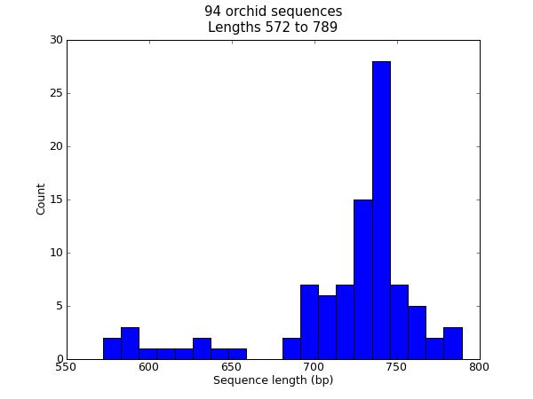
Fig. 22 Histogram of orchid sequence lengths.

That should pop up a new window containing the graph shown in Fig. 22. Notice that most of these orchid sequences are about \(740\) bp long, and there could be two distinct classes of sequence here with a subset of shorter sequences.

Tip: Rather than using pylab.show() to show the plot in a window, you can also use pylab.savefig(...) to save the figure to a file (e.g. as a PNG or PDF).

Plot of sequence GC%

Another easily calculated quantity of a nucleotide sequence is the GC%. You might want to look at the GC% of all the genes in a bacterial genome for example, and investigate any outliers which could have been recently acquired by horizontal gene transfer. Again, for this example we’ll reuse our orchid FASTA file ls_orchid.fasta.

First of all, we will use Bio.SeqIO to parse the FASTA file and compile a list of all the GC percentages. Again, you could do this with a for loop, but I prefer this:

from Bio import SeqIO
from Bio.SeqUtils import gc_fraction

gc_values = sorted(
    100 * gc_fraction(rec.seq) for rec in SeqIO.parse("ls_orchid.fasta", "fasta")
)

Having read in each sequence and calculated the GC%, we then sorted them into ascending order. Now we’ll take this list of floating point values and plot them with matplotlib:

import pylab

pylab.plot(gc_values)
pylab.title(
    "%i orchid sequences\nGC%% %0.1f to %0.1f"
    % (len(gc_values), min(gc_values), max(gc_values))
)
pylab.xlabel("Genes")
pylab.ylabel("GC%")
pylab.show()

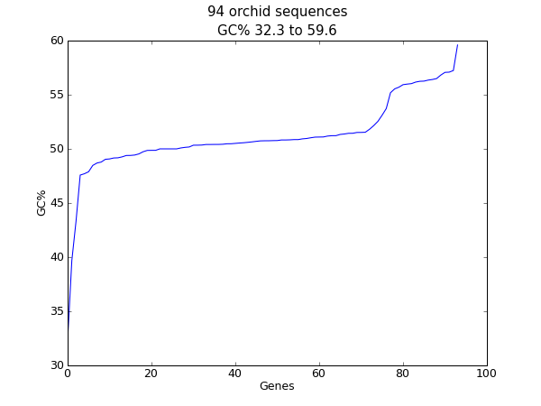
Fig. 23 Histogram of orchid sequence lengths.

As in the previous example, that should pop up a new window with the graph shown in Fig. 23. If you tried this on the full set of genes from one organism, you’d probably get a much smoother plot than this.

Nucleotide dot plots

A dot plot is a way of visually comparing two nucleotide sequences for similarity to each other. A sliding window is used to compare short sub-sequences to each other, often with a mismatch threshold. Here for simplicity we’ll only look for perfect matches (shown in black in Fig. 24).

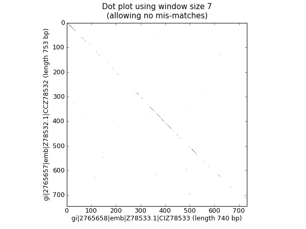
Fig. 24 Nucleotide dot plot of two orchid sequences using image show.

To start off, we’ll need two sequences. For the sake of argument, we’ll just take the first two from our orchid FASTA file ls_orchid.fasta:

from Bio import SeqIO

with open("ls_orchid.fasta") as in_handle:
    record_iterator = SeqIO.parse(in_handle, "fasta")
    rec_one = next(record_iterator)
    rec_two = next(record_iterator)

We’re going to show two approaches. Firstly, a simple naive implementation which compares all the window sized sub-sequences to each other to compiles a similarity matrix. You could construct a matrix or array object, but here we just use a list of lists of booleans created with a nested list comprehension:

window = 7
seq_one = rec_one.seq.upper()
seq_two = rec_two.seq.upper()
data = [
    [
        (seq_one[i : i + window] != seq_two[j : j + window])
        for j in range(len(seq_one) - window)
    ]
    for i in range(len(seq_two) - window)
]

Note that we have not checked for reverse complement matches here. Now we’ll use the matplotlib’s pylab.imshow() function to display this data, first requesting the gray color scheme so this is done in black and white:

import pylab

pylab.gray()
pylab.imshow(data)
pylab.xlabel("%s (length %i bp)" % (rec_one.id, len(rec_one)))
pylab.ylabel("%s (length %i bp)" % (rec_two.id, len(rec_two)))
pylab.title("Dot plot using window size %i\n(allowing no mis-matches)" % window)
pylab.show()

That should pop up a new window showing the graph in Fig. 24. As you might have expected, these two sequences are very similar with a partial line of window sized matches along the diagonal. There are no off diagonal matches which would be indicative of inversions or other interesting events.

The above code works fine on small examples, but there are two problems applying this to larger sequences, which we will address below. First off all, this brute force approach to the all against all comparisons is very slow. Instead, we’ll compile dictionaries mapping the window sized sub-sequences to their locations, and then take the set intersection to find those sub-sequences found in both sequences. This uses more memory, but is much faster. Secondly, the pylab.imshow() function is limited in the size of matrix it can display. As an alternative, we’ll use the pylab.scatter() function.

We start by creating dictionaries mapping the window-sized sub-sequences to locations:

window = 7
dict_one = {}
dict_two = {}
for seq, section_dict in [
    (rec_one.seq.upper(), dict_one),
    (rec_two.seq.upper(), dict_two),
]:
    for i in range(len(seq) - window):
        section = seq[i : i + window]
        try:
            section_dict[section].append(i)
        except KeyError:
            section_dict[section] = [i]
# Now find any sub-sequences found in both sequences
matches = set(dict_one).intersection(dict_two)
print("%i unique matches" % len(matches))

In order to use the pylab.scatter() we need separate lists for the \(x\) and \(y\) coordinates:

# Create lists of x and y coordinates for scatter plot
x = []
y = []
for section in matches:
    for i in dict_one[section]:
        for j in dict_two[section]:
            x.append(i)
            y.append(j)

We are now ready to draw the revised dot plot as a scatter plot:

import pylab

pylab.cla()  # clear any prior graph
pylab.gray()
pylab.scatter(x, y)
pylab.xlim(0, len(rec_one) - window)
pylab.ylim(0, len(rec_two) - window)
pylab.xlabel("%s (length %i bp)" % (rec_one.id, len(rec_one)))
pylab.ylabel("%s (length %i bp)" % (rec_two.id, len(rec_two)))
pylab.title("Dot plot using window size %i\n(allowing no mis-matches)" % window)
pylab.show()

That should pop up a new window showing the graph in Fig. 25.

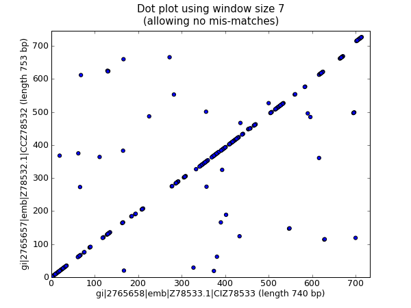
Fig. 25 Nucleotide dot plot of two orchid sequence using scatter.

Personally I find this second plot much easier to read! Again note that we have not checked for reverse complement matches here – you could extend this example to do this, and perhaps plot the forward matches in one color and the reverse matches in another.

Plotting the quality scores of sequencing read data

If you are working with second generation sequencing data, you may want to try plotting the quality data. Here is an example using two FASTQ files containing paired end reads, SRR001666_1.fastq for the forward reads, and SRR001666_2.fastq for the reverse reads. These were downloaded from the ENA sequence read archive FTP site (ftp://ftp.sra.ebi.ac.uk/vol1/fastq/SRR001/SRR001666/SRR001666_1.fastq.gz and ftp://ftp.sra.ebi.ac.uk/vol1/fastq/SRR001/SRR001666/SRR001666_2.fastq.gz), and are from E. coli – see https://www.ebi.ac.uk/ena/data/view/SRR001666 for details.

In the following code the pylab.subplot(...) function is used in order to show the forward and reverse qualities on two subplots, side by side. There is also a little bit of code to only plot the first fifty reads.

import pylab
from Bio import SeqIO

for subfigure in [1, 2]:
    filename = "SRR001666_%i.fastq" % subfigure
    pylab.subplot(1, 2, subfigure)
    for i, record in enumerate(SeqIO.parse(filename, "fastq")):
        if i >= 50:
            break  # trick!
        pylab.plot(record.letter_annotations["phred_quality"])
    pylab.ylim(0, 45)
    pylab.ylabel("PHRED quality score")
    pylab.xlabel("Position")
pylab.savefig("SRR001666.png")
print("Done")

You should note that we are using the Bio.SeqIO format name fastq here because the NCBI has saved these reads using the standard Sanger FASTQ format with PHRED scores. However, as you might guess from the read lengths, this data was from an Illumina Genome Analyzer and was probably originally in one of the two Solexa/Illumina FASTQ variant file formats instead.

This example uses the pylab.savefig(...) function instead of pylab.show(...), but as mentioned before both are useful.

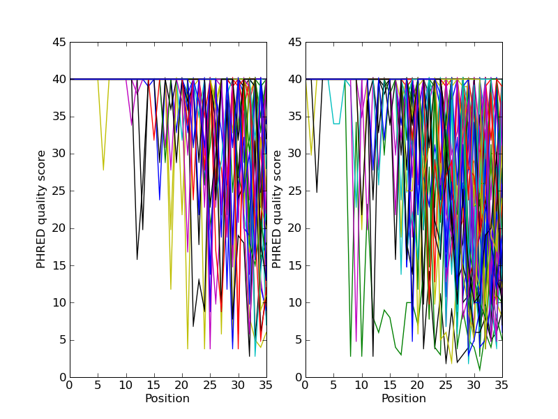
Fig. 26 Quality plot for some paired end reads.

The result is shown in Fig. 26.

BioSQL – storing sequences in a relational database

BioSQL is a joint effort between the OBF projects (BioPerl, BioJava etc) to support a shared database schema for storing sequence data. In theory, you could load a GenBank file into the database with BioPerl, then using Biopython extract this from the database as a record object with features - and get more or less the same thing as if you had loaded the GenBank file directly as a SeqRecord using Bio.SeqIO (Chapter Sequence Input/Output).

Biopython’s BioSQL module is currently documented at http://biopython.org/wiki/BioSQL which is part of our wiki pages.