Going 3D: The PDB module
Bio.PDB is a Biopython module that focuses on working with crystal structures of biological macromolecules. Among other things, Bio.PDB includes a PDBParser class that produces a Structure object, which can be used to access the atomic data in the file in a convenient manner. There is limited support for parsing the information contained in the PDB header. PDB file format is no longer being modified or extended to support new content and PDBx/mmCIF became the standard PDB archive format in 2014. All the Worldwide Protein Data Bank (wwPDB) sites uses the macromolecular Crystallographic Information File (mmCIF) data dictionaries to describe the information content of PDB entries. mmCIF uses a flexible and extensible key-value pair format for representing macromolecular structural data and imposes no limitations for the number of atoms, residues or chains that can be represented in a single PDB entry (no split entries!).
Reading and writing crystal structure files
Reading an mmCIF file
First create an MMCIFParser object:
>>> from Bio.PDB.MMCIFParser import MMCIFParser
>>> parser = MMCIFParser()
Then use this parser to create a structure object from the mmCIF file:
>>> structure = parser.get_structure("1fat", "1fat.cif")
To have some more low level access to an mmCIF file, you can use the
MMCIF2Dict class to create a Python dictionary that maps all mmCIF
tags in an mmCIF file to their values. Whether there are multiple values
(like in the case of tag _atom_site.Cartn_y, which holds the
\(y\) coordinates of all atoms) or a single value (like the initial
deposition date), the tag is mapped to a list of values. The dictionary
is created from the mmCIF file as follows:
>>> from Bio.PDB.MMCIF2Dict import MMCIF2Dict
>>> mmcif_dict = MMCIF2Dict("1FAT.cif")
Example: get the solvent content from an mmCIF file:
>>> sc = mmcif_dict["_exptl_crystal.density_percent_sol"]
Example: get the list of the \(y\) coordinates of all atoms
>>> y_list = mmcif_dict["_atom_site.Cartn_y"]
Reading a BinaryCIF file
Create a BinaryCIFParser object:
>>> from Bio.PDB.binary_cif import BinaryCIFParser
>>> parser = BinaryCIFParser()
Call get_structure with the path to the BinaryCIF file:
>>> parser.get_structure("1GBT", "1gbt.bcif.gz")
<Structure id=1GBT>
Reading files in the MMTF format
You can use the direct MMTFParser to read a structure from a file:
>>> from Bio.PDB.mmtf import MMTFParser
>>> structure = MMTFParser.get_structure("PDB/4CUP.mmtf")
Or you can use the same class to get a structure by its PDB ID:
>>> structure = MMTFParser.get_structure_from_url("4CUP")
This gives you a Structure object as if read from a PDB or mmCIF file.
You can also have access to the underlying data using the external MMTF library which Biopython is using internally:
>>> from mmtf import fetch
>>> decoded_data = fetch("4CUP")
For example you can access just the X-coordinate.
>>> print(decoded_data.x_coord_list)
Reading a PDB file
First we create a PDBParser object:
>>> from Bio.PDB.PDBParser import PDBParser
>>> parser = PDBParser(PERMISSIVE=1)
The PERMISSIVE flag indicates that a number of common problems (see
Examples) associated with PDB files will be
ignored (but note that some atoms and/or residues will be missing). If
the flag is not present a PDBConstructionException will be generated
if any problems are detected during the parse operation.
The Structure object is then produced by letting the PDBParser
object parse a PDB file (the PDB file in this case is called
pdb1fat.ent, 1fat is a user defined name for the structure):
>>> structure_id = "1fat"
>>> filename = "pdb1fat.ent"
>>> structure = parser.get_structure(structure_id, filename)
You can extract the header and trailer (simple lists of strings) of the
PDB file from the PDBParser object with the get_header and
get_trailer methods. Note however that many PDB files contain
headers with incomplete or erroneous information. Many of the errors
have been fixed in the equivalent mmCIF files. Hence, if you are
interested in the header information, it is a good idea to extract
information from mmCIF files using the ``MMCIF2Dict`` tool described
above, instead of parsing the PDB header.
Now that is clarified, let’s return to parsing the PDB header. The
structure object has an attribute called header which is a Python
dictionary that maps header records to their values.
Example:
>>> resolution = structure.header["resolution"]
>>> keywords = structure.header["keywords"]
The available keys are name, head, deposition_date,
release_date, structure_method, resolution,
structure_reference (which maps to a list of references),
journal_reference, author, compound (which maps to a
dictionary with various information about the crystallized compound),
has_missing_residues, missing_residues, and astral (which
maps to dictionary with additional information about the domain if
present).
has_missing_residues maps to a bool that is True if at least one
non-empty REMARK 465 header line was found. In this case you should
assume that the molecule used in the experiment has some residues for
which no ATOM coordinates could be determined. missing_residues maps
to a list of dictionaries with information about the missing residues.
The list of missing residues will be empty or incomplete if the PDB
header does not follow the template from the PDB specification.
The dictionary can also be created without creating a Structure
object, ie. directly from the PDB file:
>>> from Bio.PDB import parse_pdb_header
>>> with open(filename, "r") as handle:
...     header_dict = parse_pdb_header(handle)
...
Reading a PQR file
In order to parse a PQR file, proceed in a similar manner as in the case of PDB files:
Create a PDBParser object, using the is_pqr flag:
>>> from Bio.PDB.PDBParser import PDBParser
>>> pqr_parser = PDBParser(PERMISSIVE=1, is_pqr=True)
The is_pqr flag set to True indicates that the file to be parsed
is a PQR file, and that the parser should read the atomic charge and
radius fields for each atom entry. Following the same procedure as for
PQR files, a Structure object is then produced, and the PQR file is
parsed.
>>> structure_id = "1fat"
>>> filename = "pdb1fat.ent"
>>> structure = parser.get_structure(structure_id, filename, is_pqr=True)
Reading a PDBML (PDB XML) file
Create a PDBMLParser object:
>>> from Bio.PDB.PDBMLParser import PDBMLParser
>>> pdbml_parser = PDBMLParser()
Call get_structure with a file path or file object containing the PDB structure in XML format:
>>> structure = pdbml_parser.get_structure("1GBT.xml")
Writing mmCIF files
The MMCIFIO class can be used to write structures to the mmCIF file
format:
>>> io = MMCIFIO()
>>> io.set_structure(s)
>>> io.save("out.cif")
The Select class can be used in a similar way to PDBIO below.
mmCIF dictionaries read using MMCIF2Dict can also be written:
>>> io = MMCIFIO()
>>> io.set_dict(d)
>>> io.save("out.cif")
Writing PDB files
Use the PDBIO class for this. It’s easy to write out specific parts
of a structure too, of course.
Example: saving a structure
>>> io = PDBIO()
>>> io.set_structure(s)
>>> io.save("out.pdb")
If you want to write out a part of the structure, make use of the
Select class (also in PDBIO). Select has four methods:
accept_model(model)accept_chain(chain)accept_residue(residue)accept_atom(atom)
By default, every method returns 1 (which means the
model/chain/residue/atom is included in the output). By subclassing
Select and returning 0 when appropriate you can exclude models,
chains, etc. from the output. Cumbersome maybe, but very powerful. The
following code only writes out glycine residues:
>>> class GlySelect(Select):
...     def accept_residue(self, residue):
...         if residue.get_name() == "GLY":
...             return True
...         else:
...             return False
...
>>> io = PDBIO()
>>> io.set_structure(s)
>>> io.save("gly_only.pdb", GlySelect())
If this is all too complicated for you, the Dice module contains a
handy extract function that writes out all residues in a chain
between a start and end residue.
Writing PQR files
Use the PDBIO class as you would for a PDB file, with the flag
is_pqr=True. The PDBIO methods can be used in the case of PQR files
as well.
Example: writing a PQR file
>>> io = PDBIO(is_pqr=True)
>>> io.set_structure(s)
>>> io.save("out.pdb")
Writing MMTF files
To write structures to the MMTF file format:
>>> from Bio.PDB.mmtf import MMTFIO
>>> io = MMTFIO()
>>> io.set_structure(s)
>>> io.save("out.mmtf")
The Select class can be used as above. Note that the bonding
information, secondary structure assignment and some other information
contained in standard MMTF files is not written out as it is not easy to
determine from the structure object. In addition, molecules that are
grouped into the same entity in standard MMTF files are treated as
separate entities by MMTFIO.
Structure representation
The overall layout of a Structure object follows the so-called SMCRA
(Structure/Model/Chain/Residue/Atom) architecture:
A structure consists of models
A model consists of chains
A chain consists of residues
A residue consists of atoms
This is the way many structural biologists/bioinformaticians think about
structure, and provides a simple but efficient way to deal with
structure. Additional stuff is essentially added when needed. A UML
diagram of the Structure object (forget about the Disordered
classes for now) is shown in Fig. 3. Such a data
structure is not necessarily best suited for the representation of the
macromolecular content of a structure, but it is absolutely necessary
for a good interpretation of the data present in a file that describes
the structure (typically a PDB or MMCIF file). If this hierarchy cannot
represent the contents of a structure file, it is fairly certain that
the file contains an error or at least does not describe the structure
unambiguously. If a SMCRA data structure cannot be generated, there is
reason to suspect a problem. Parsing a PDB file can thus be used to
detect likely problems. We will give several examples of this in section
Examples.
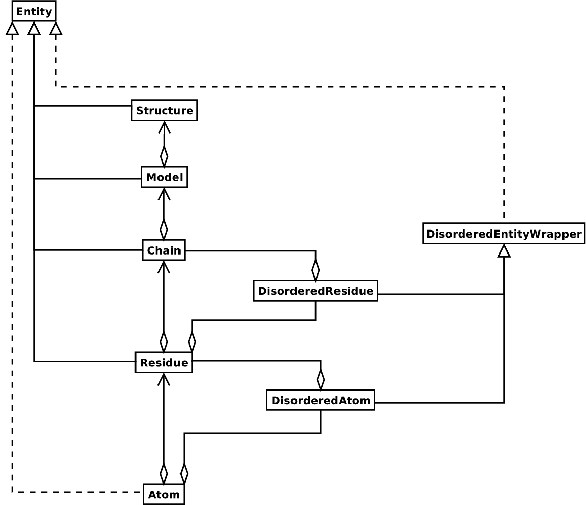
Fig. 3 UML diagram of SMCRA architecture of the Structure class.
This is used to represent a macromolecular structure. Full lines with diamonds denote aggregation, full lines with arrows denote referencing, full lines with triangles denote inheritance and dashed lines with triangles denote interface realization.
Structure, Model, Chain and Residue are all subclasses of the Entity base class. The Atom class only (partly) implements the Entity interface (because an Atom does not have children).
For each Entity subclass, you can extract a child by using a unique id for that child as a key (e.g. you can extract an Atom object from a Residue object by using an atom name string as a key, you can extract a Chain object from a Model object by using its chain identifier as a key).
Disordered atoms and residues are represented by DisorderedAtom and DisorderedResidue classes, which are both subclasses of the DisorderedEntityWrapper base class. They hide the complexity associated with disorder and behave exactly as Atom and Residue objects.
In general, a child Entity object (i.e. Atom, Residue, Chain, Model) can be extracted from its parent (i.e. Residue, Chain, Model, Structure, respectively) by using an id as a key.
>>> child_entity = parent_entity[child_id]
You can also get a list of all child Entities of a parent Entity object. Note that this list is sorted in a specific way (e.g. according to chain identifier for Chain objects in a Model object).
>>> child_list = parent_entity.get_list()
You can also get the parent from a child:
>>> parent_entity = child_entity.get_parent()
At all levels of the SMCRA hierarchy, you can also extract a full id. The full id is a tuple containing all id’s starting from the top object (Structure) down to the current object. A full id for a Residue object e.g. is something like:
>>> full_id = residue.get_full_id()
>>> print(full_id)
("1abc", 0, "A", ("", 10, "A"))
This corresponds to:
The Structure with id
"1abc"The Model with id
0The Chain with id
"A"The Residue with id
("", 10, "A")
The Residue id indicates that the residue is not a hetero-residue (nor a
water) because it has a blank hetero field, that its sequence identifier
is 10 and that its insertion code is "A".
To get the entity’s id, use the get_id method:
>>> entity.get_id()
You can check if the entity has a child with a given id by using the
has_id method:
>>> entity.has_id(entity_id)
The length of an entity is equal to its number of children:
>>> nr_children = len(entity)
It is possible to delete, rename, add, etc. child entities from a parent entity, but this does not include any sanity checks (e.g. it is possible to add two residues with the same id to one chain). This really should be done via a nice Decorator class that includes integrity checking, but you can take a look at the code (Entity.py) if you want to use the raw interface.
Structure
The Structure object is at the top of the hierarchy. Its id is a user given string. The Structure contains a number of Model children. Most crystal structures (but not all) contain a single model, while NMR structures typically consist of several models. Disorder in crystal structures of large parts of molecules can also result in several models.
Model
The id of the Model object is an integer, which is derived from the
position of the model in the parsed file (they are automatically
numbered starting from 0). Crystal structures generally have only one
model (with id 0), while NMR files usually have several models. Whereas
many PDB parsers assume that there is only one model, the Structure
class in Bio.PDB is designed such that it can easily handle PDB
files with more than one model.
As an example, to get the first model from a Structure object, use
>>> first_model = structure[0]
The Model object stores a list of Chain children.
Chain
The id of a Chain object is derived from the chain identifier in the PDB/mmCIF file, and is a single character (typically a letter). Each Chain in a Model object has a unique id. As an example, to get the Chain object with identifier “A” from a Model object, use
>>> chain_A = model["A"]
The Chain object stores a list of Residue children.
Residue
A residue id is a tuple with three elements:
The hetero-field (hetfield): this is
'W'in the case of a water molecule;'H_'followed by the residue name for other hetero residues (e.g.'H_GLC'in the case of a glucose molecule);blank for standard amino and nucleic acids.
This scheme is adopted for reasons described in section Associated problems.
The sequence identifier (resseq), an integer describing the position of the residue in the chain (e.g., 100);
The insertion code (icode); a string, e.g. ’A’. The insertion code is sometimes used to preserve a certain desirable residue numbering scheme. A Ser 80 insertion mutant (inserted e.g. between a Thr 80 and an Asn 81 residue) could e.g. have sequence identifiers and insertion codes as follows: Thr 80 A, Ser 80 B, Asn 81. In this way the residue numbering scheme stays in tune with that of the wild type structure.
The id of the above glucose residue would thus be
(’H_GLC’, 100, ’A’). If the hetero-flag and insertion code are
blank, the sequence identifier alone can be used:
# Full id
>>> residue = chain[(" ", 100, " ")]
# Shortcut id
>>> residue = chain[100]
The reason for the hetero-flag is that many, many PDB files use the same sequence identifier for an amino acid and a hetero-residue or a water, which would create obvious problems if the hetero-flag was not used.
Unsurprisingly, a Residue object stores a set of Atom children. It also contains a string that specifies the residue name (e.g. “ASN”) and the segment identifier of the residue (well known to X-PLOR users, but not used in the construction of the SMCRA data structure).
Let’s look at some examples. Asn 10 with a blank insertion code would
have residue id (’ ’, 10, ’ ’). Water 10 would have residue id
(’W’, 10, ’ ’). A glucose molecule (a hetero residue with residue
name GLC) with sequence identifier 10 would have residue id
(’H_GLC’, 10, ’ ’). In this way, the three residues (with the same
insertion code and sequence identifier) can be part of the same chain
because their residue id’s are distinct.
In most cases, the hetflag and insertion code fields will be blank, e.g.
(’ ’, 10, ’ ’). In these cases, the sequence identifier can be used
as a shortcut for the full id:
# use full id
>>> res10 = chain[(" ", 10, " ")]
# use shortcut
>>> res10 = chain[10]
Each Residue object in a Chain object should have a unique id. However, disordered residues are dealt with in a special way, as described in section Point mutations.
A Residue object has a number of additional methods:
>>> residue.get_resname()  # returns the residue name, e.g. "ASN"
>>> residue.is_disordered()  # returns 1 if the residue has disordered atoms
>>> residue.get_segid()  # returns the SEGID, e.g. "CHN1"
>>> residue.has_id(name)  # test if a residue has a certain atom
You can use is_aa(residue) to test if a Residue object is an amino
acid.
Atom
The Atom object stores the data associated with an atom, and has no children. The id of an atom is its atom name (e.g. “OG” for the side chain oxygen of a Ser residue). An Atom id needs to be unique in a Residue. Again, an exception is made for disordered atoms, as described in section Disordered atoms.
The atom id is simply the atom name (eg. ’CA’). In practice, the
atom name is created by stripping all spaces from the atom name in the
PDB file.
However, in PDB files, a space can be part of an atom name. Often,
calcium atoms are called ’CA..’ in order to distinguish them from
C\(\alpha\) atoms (which are called ’.CA.’). In cases were
stripping the spaces would create problems (ie. two atoms called
’CA’ in the same residue) the spaces are kept.
In a PDB file, an atom name consists of 4 chars, typically with leading and trailing spaces. Often these spaces can be removed for ease of use (e.g. an amino acid C\(\alpha\) atom is labeled “.CA.” in a PDB file, where the dots represent spaces). To generate an atom name (and thus an atom id) the spaces are removed, unless this would result in a name collision in a Residue (i.e. two Atom objects with the same atom name and id). In the latter case, the atom name including spaces is tried. This situation can e.g. happen when one residue contains atoms with names “.CA.” and “CA..”, although this is not very likely.
The atomic data stored includes the atom name, the atomic coordinates (including standard deviation if present), the B factor (including anisotropic B factors and standard deviation if present), the altloc specifier and the full atom name including spaces. Less used items like the atom element number or the atomic charge sometimes specified in a PDB file are not stored.
To manipulate the atomic coordinates, use the transform method of
the Atom object. Use the set_coord method to specify the atomic
coordinates directly.
An Atom object has the following additional methods:
>>> a.get_name()  # atom name (spaces stripped, e.g. "CA")
>>> a.get_id()  # id (equals atom name)
>>> a.get_coord()  # atomic coordinates
>>> a.get_vector()  # atomic coordinates as Vector object
>>> a.get_bfactor()  # isotropic B factor
>>> a.get_occupancy()  # occupancy
>>> a.get_altloc()  # alternative location specifier
>>> a.get_sigatm()  # standard deviation of atomic parameters
>>> a.get_siguij()  # standard deviation of anisotropic B factor
>>> a.get_anisou()  # anisotropic B factor
>>> a.get_fullname()  # atom name (with spaces, e.g. ".CA.")
To represent the atom coordinates, siguij, anisotropic B factor and sigatm Numpy arrays are used.
The get_vector method returns a Vector object representation of
the coordinates of the Atom object, allowing you to do vector
operations on atomic coordinates. Vector implements the full set of
3D vector operations, matrix multiplication (left and right) and some
advanced rotation-related operations as well.
As an example of the capabilities of Bio.PDB’s Vector module,
suppose that you would like to find the position of a Gly residue’s
C\(\beta\) atom, if it had one. Rotating the N atom of the Gly
residue along the C\(\alpha\)-C bond over -120 degrees roughly
puts it in the position of a virtual C\(\beta\) atom. Here’s how
to do it, making use of the rotaxis method (which can be used to
construct a rotation around a certain axis) of the Vector module:
# get atom coordinates as vectors
>>> n = residue["N"].get_vector()
>>> c = residue["C"].get_vector()
>>> ca = residue["CA"].get_vector()
# center at origin
>>> n = n - ca
>>> c = c - ca
# find rotation matrix that rotates n
# -120 degrees along the ca-c vector
>>> rot = rotaxis(-pi * 120.0 / 180.0, c)
# apply rotation to ca-n vector
>>> cb_at_origin = n.left_multiply(rot)
# put on top of ca atom
>>> cb = cb_at_origin + ca
This example shows that it’s possible to do some quite nontrivial vector
operations on atomic data, which can be quite useful. In addition to all
the usual vector operations (cross (use **), and dot (use
*) product, angle, norm, etc.) and the above mentioned rotaxis
function, the Vector module also has methods to rotate (rotmat)
or reflect (refmat) one vector on top of another.
Extracting a specific Atom/Residue/Chain/Model from a Structure
These are some examples:
>>> model = structure[0]
>>> chain = model["A"]
>>> residue = chain[100]
>>> atom = residue["CA"]
Note that you can use a shortcut:
>>> atom = structure[0]["A"][100]["CA"]
Disorder
Bio.PDB can handle both disordered atoms and point mutations (i.e. a Gly and an Ala residue in the same position).
General approach
Disorder should be dealt with from two points of view: the atom and the residue points of view. In general, we have tried to encapsulate all the complexity that arises from disorder. If you just want to loop over all C\(\alpha\) atoms, you do not care that some residues have a disordered side chain. On the other hand it should also be possible to represent disorder completely in the data structure. Therefore, disordered atoms or residues are stored in special objects that behave as if there is no disorder. This is done by only representing a subset of the disordered atoms or residues. Which subset is picked (e.g. which of the two disordered OG side chain atom positions of a Ser residue is used) can be specified by the user.
Disordered atoms
Disordered atoms are represented by ordinary Atom objects, but all
Atom objects that represent the same physical atom are stored in a
DisorderedAtom object (see Fig. 3). Each
Atom object in a DisorderedAtom object can be uniquely indexed
using its altloc specifier. The DisorderedAtom object forwards all
uncaught method calls to the selected Atom object, by default the one
that represents the atom with the highest occupancy. The user can of
course change the selected Atom object, making use of its altloc
specifier. In this way atom disorder is represented correctly without
much additional complexity. In other words, if you are not interested in
atom disorder, you will not be bothered by it.
Each disordered atom has a characteristic altloc identifier. You can
specify that a DisorderedAtom object should behave like the Atom
object associated with a specific altloc identifier:
>>> atom.disordered_select("A")  # select altloc A atom
>>> print(atom.get_altloc())
"A"
>>> atom.disordered_select("B")  # select altloc B atom
>>> print(atom.get_altloc())
"B"
Disordered residues
Common case
The most common case is a residue that contains one or more disordered atoms. This is evidently solved by using DisorderedAtom objects to represent the disordered atoms, and storing the DisorderedAtom object in a Residue object just like ordinary Atom objects. The DisorderedAtom will behave exactly like an ordinary atom (in fact the atom with the highest occupancy) by forwarding all uncaught method calls to one of the Atom objects (the selected Atom object) it contains.
Point mutations
A special case arises when disorder is due to a point mutation, i.e. when two or more point mutants of a polypeptide are present in the crystal. An example of this can be found in PDB structure 1EN2.
Since these residues belong to a different residue type (e.g. let’s say
Ser 60 and Cys 60) they should not be stored in a single Residue
object as in the common case. In this case, each residue is represented
by one Residue object, and both Residue objects are stored in a
single DisorderedResidue object (see Fig. 3).
The DisorderedResidue object forwards all uncaught methods to the
selected Residue object (by default the last Residue object
added), and thus behaves like an ordinary residue. Each Residue
object in a DisorderedResidue object can be uniquely identified by
its residue name. In the above example, residue Ser 60 would have id
“SER” in the DisorderedResidue object, while residue Cys 60 would
have id “CYS”. The user can select the active Residue object in a
DisorderedResidue object via this id.
Example: suppose that a chain has a point mutation at position 10, consisting of a Ser and a Cys residue. Make sure that residue 10 of this chain behaves as the Cys residue.
>>> residue = chain[10]
>>> residue.disordered_select("CYS")
In addition, you can get a list of all Atom objects (ie. all
DisorderedAtom objects are ’unpacked’ to their individual Atom
objects) using the get_unpacked_list method of a
(Disordered)Residue object.
Hetero residues
Associated problems
A common problem with hetero residues is that several hetero and non-hetero residues present in the same chain share the same sequence identifier (and insertion code). Therefore, to generate a unique id for each hetero residue, waters and other hetero residues are treated in a different way.
Remember that Residue object have the tuple (hetfield, resseq, icode) as id. The hetfield is blank (“ ”) for amino and nucleic acids, and a string for waters and other hetero residues. The content of the hetfield is explained below.
Water residues
The hetfield string of a water residue consists of the letter “W”. So a typical residue id for a water is (“W”, 1, “ ”).
Other hetero residues
The hetfield string for other hetero residues starts with “H_” followed by the residue name. A glucose molecule e.g. with residue name “GLC” would have hetfield “H_GLC”. Its residue id could e.g. be (“H_GLC”, 1, “ ”).
Analyzing structures
Measuring distances
The minus operator for atoms has been overloaded to return the distance between two atoms.
# Get some atoms
>>> ca1 = residue1["CA"]
>>> ca2 = residue2["CA"]
# Simply subtract the atoms to get their distance
>>> distance = ca1 - ca2
Measuring angles
Use the vector representation of the atomic coordinates, and the
calc_angle function from the Vector module:
>>> vector1 = atom1.get_vector()
>>> vector2 = atom2.get_vector()
>>> vector3 = atom3.get_vector()
>>> angle = calc_angle(vector1, vector2, vector3)
Measuring torsion angles
Use the vector representation of the atomic coordinates, and the
calc_dihedral function from the Vector module:
>>> vector1 = atom1.get_vector()
>>> vector2 = atom2.get_vector()
>>> vector3 = atom3.get_vector()
>>> vector4 = atom4.get_vector()
>>> angle = calc_dihedral(vector1, vector2, vector3, vector4)
Internal coordinates - distances, angles, torsion angles, distance plots, etc
Protein structures are normally supplied in 3D XYZ coordinates relative
to a fixed origin, as in a PDB or mmCIF file. The internal_coords
module facilitates converting this system to and from bond lengths,
angles and dihedral angles. In addition to supporting standard psi,
phi, chi, etc. calculations on protein structures, this representation
is invariant to translation and rotation, and the implementation exposes
multiple benefits for structure analysis.
First load up some modules here for later examples:
>>> from Bio.PDB.PDBParser import PDBParser
>>> from Bio.PDB.Chain import Chain
>>> from Bio.PDB.internal_coords import *
>>> from Bio.PDB.PICIO import write_PIC, read_PIC, read_PIC_seq
>>> from Bio.PDB.ic_rebuild import write_PDB, IC_duplicate, structure_rebuild_test
>>> from Bio.PDB.SCADIO import write_SCAD
>>> from Bio.Seq import Seq
>>> from Bio.SeqRecord import SeqRecord
>>> from Bio.PDB.PDBIO import PDBIO
>>> import numpy as np
Accessing dihedrals, angles and bond lengths
We start with the simple case of computing internal coordinates for a structure:
>>> # load a structure as normal, get first chain
>>> parser = PDBParser()
>>> myProtein = parser.get_structure("1a8o", "1A8O.pdb")
>>> myChain = myProtein[0]["A"]
>>> # compute bond lengths, angles, dihedral angles
>>> myChain.atom_to_internal_coordinates(verbose=True)
chain break at THR  186  due to MaxPeptideBond (1.4 angstroms) exceeded
chain break at THR  216  due to MaxPeptideBond (1.4 angstroms) exceeded
The chain break warnings for 1A8O are suppressed by removing the
verbose=True option above. To avoid the creation of a break and
instead allow unrealistically long N-C bonds, override the class
variable MaxPeptideBond, e.g.:
>>> IC_Chain.MaxPeptideBond = 4.0
>>> myChain.internal_coord = None  # force re-loading structure data with new cutoff
>>> myChain.atom_to_internal_coordinates(verbose=True)
At this point the values are available at both the chain and residue level. The first residue of 1A8O is HETATM MSE (selenomethionine), so we investigate residue 2 below using either canonical names or atom specifiers. Here we obtain the chi1 dihedral and tau angles by name and by atom sequence, and the C\(\alpha\)-C\(\beta\) distance by specifying the atom pair:
>>> r2 = myChain.child_list[1]
>>> r2
<Residue ASP het=  resseq=152 icode= >
>>> r2ic = r2.internal_coord
>>> print(r2ic, ":", r2ic.pretty_str(), ":", r2ic.rbase, ":", r2ic.lc)
('1a8o', 0, 'A', (' ', 152, ' ')) : ASP  152  : (152, None, 'D') : D
>>> r2chi1 = r2ic.get_angle("chi1")
>>> print(round(r2chi1, 2))
-144.86
>>> r2ic.get_angle("chi1") == r2ic.get_angle("N:CA:CB:CG")
True
>>> print(round(r2ic.get_angle("tau"), 2))
113.45
>>> r2ic.get_angle("tau") == r2ic.get_angle("N:CA:C")
True
>>> print(round(r2ic.get_length("CA:CB"), 2))
1.53
The Chain.internal_coord object holds arrays and dictionaries of
hedra (3 bonded atoms) and dihedra (4 bonded atoms) objects. The
dictionaries are indexed by tuples of AtomKey objects; AtomKey
objects capture residue position, insertion code, 1 or 3-character
residue name, atom name, altloc and occupancy.
Below we obtain the same chi1 and tau angles as above by indexing
the Chain arrays directly, using AtomKeys to index the
Chain arrays:
>>> myCic = myChain.internal_coord

>>> r2chi1_object = r2ic.pick_angle("chi1")
>>> # or same thing (as for get_angle() above):
>>> r2chi1_object == r2ic.pick_angle("N:CA:CB:CG")
True
>>> r2chi1_key = r2chi1_object.atomkeys
>>> r2chi1_key  # r2chi1_key is tuple of AtomKeys
(152_D_N, 152_D_CA, 152_D_CB, 152_D_CG)

>>> r2chi1_index = myCic.dihedraNdx[r2chi1_key]
>>> # or same thing:
>>> r2chi1_index == r2chi1_object.ndx
True
>>> print(round(myCic.dihedraAngle[r2chi1_index], 2))
-144.86
>>> # also:
>>> r2chi1_object == myCic.dihedra[r2chi1_key]
True

>>> # hedra angles are similar:
>>> r2tau = r2ic.pick_angle("tau")
>>> print(round(myCic.hedraAngle[r2tau.ndx], 2))
113.45
Obtaining bond length data at the Chain level is more complicated
(and not recommended). As shown here, multiple hedra will share a single
bond in different positions:
>>> r2CaCb = r2ic.pick_length("CA:CB")  # returns list of hedra containing bond
>>> r2CaCb[0][0].atomkeys
(152_D_CB, 152_D_CA, 152_D_C)
>>> print(round(myCic.hedraL12[r2CaCb[0][0].ndx], 2))  # position 1-2
1.53
>>> r2CaCb[0][1].atomkeys
(152_D_N, 152_D_CA, 152_D_CB)
>>> print(round(myCic.hedraL23[r2CaCb[0][1].ndx], 2))  # position 2-3
1.53
>>> r2CaCb[0][2].atomkeys
(152_D_CA, 152_D_CB, 152_D_CG)
>>> print(round(myCic.hedraL12[r2CaCb[0][2].ndx], 2))  # position 1-2
1.53
Please use the Residue level set_length:math:`` function
instead.
Testing structures for completeness
Missing atoms and other issues can cause problems when rebuilding a
structure. Use structure_rebuild_test:math:`` to determine quickly
if a structure has sufficient data for a clean rebuild. Add
verbose=True and/or inspect the result dictionary for more detail:
>>> # check myChain makes sense (can get angles and rebuild same structure)
>>> resultDict = structure_rebuild_test(myChain)
>>> resultDict["pass"]
True
Modifying and rebuilding structures
It’s preferable to use the residue level set_angle:math:`` and
set_length:math:`` facilities for modifying internal coordinates
rather than directly accessing the Chain structures. While directly
modifying hedra angles is safe, bond lengths appear in multiple
overlapping hedra as noted above, and this is handled by
set_length:math:. When applied to a dihedral angle,
``set_angle:math:`` will wrap the result to +/-180 and rotate
adjacent dihedra as well (such as both bonds for an isoleucine chi1
angle - which is probably what you want).
>>> # rotate residue 2 chi1 angle by -120 degrees
>>> r2ic.set_angle("chi1", r2chi1 - 120.0)
>>> print(round(r2ic.get_angle("chi1"), 2))
95.14
>>> r2ic.set_length("CA:CB", 1.49)
>>> print(round(myCic.hedraL12[r2CaCb[0][0].ndx], 2))  # Cb-Ca-C position 1-2
1.49
Rebuilding a structure from internal coordinates is a simple call to
internal_to_atom_coordinates():
>>> myChain.internal_to_atom_coordinates()

>>> # just for proof:
>>> myChain.internal_coord = None  # all internal_coord data removed, only atoms left
>>> myChain.atom_to_internal_coordinates()  # re-generate internal coordinates
>>> r2ic = myChain.child_list[1].internal_coord
>>> print(round(r2ic.get_angle("chi1"), 2))  # show measured values match what was set above
95.14
>>> print(round(myCic.hedraL23[r2CaCb[0][1].ndx], 2))  # N-Ca-Cb position 2-3
1.49
The generated structure can be written with PDBIO, as normal:
write_PDB(myProtein, "myChain.pdb")
# or just the ATOM records without headers:
io = PDBIO()
io.set_structure(myProtein)
io.save("myChain2.pdb")
Protein Internal Coordinate (.pic) files and default values
A file format is defined in the PICIO module to describe protein
chains as hedra and dihedra relative to initial coordinates. All parts
of the file other than the residue sequence information (e.g.
(’1A8O’, 0, ’A’, (’ ’, 153, ’ ’)) ILE) are optional, and will be
filled in with default values if not specified and
read_PIC:math:`` is called with the defaults=True option.
Default values are calculated from Sep 2019 Dunbrack
cullpdb_pc20_res2.2_R1.0.
Here we write ‘myChain’ as a .pic file of internal coordinate
specifications and then read it back in as ‘myProtein2’.
# write chain as 'protein internal coordinates' (.pic) file
write_PIC(myProtein, "myChain.pic")
# read .pic file
myProtein2 = read_PIC("myChain.pic")
As all internal coordinate values can be replaced with defaults,
PICIO.read_PIC_seq:math:`` is supplied as a utility function to
create a valid (mostly helical) default structure from an input
sequence:
# create default structure for random sequence by reading as .pic file
myProtein3 = read_PIC_seq(
    SeqRecord(
        Seq("GAVLIMFPSTCNQYWDEHKR"),
        id="1RND",
        description="my random sequence",
    )
)
myProtein3.internal_to_atom_coordinates()
write_PDB(myProtein3, "myRandom.pdb")
It may be of interest to explore the accuracy required in e.g. omega
angles (180.0), hedra angles and/or bond lengths when generating
structures from internal coordinates. The picFlags option to
write_PIC:math:`` enables this, allowing the selection of data to
be written to the .pic file vs. left unspecified to get default values.
Various combinations are possible and some presets are supplied, for
example classic will write only psi, phi, tau, proline omega and
sidechain chi angles to the .pic file:
write_PIC(myProtein, "myChain.pic", picFlags=IC_Residue.pic_flags.classic)
myProtein2 = read_PIC("myChain.pic", defaults=True)
Accessing the all-atom AtomArray
All 3D XYZ coordinates in Biopython Atom objects are moved to a
single large array in the Chain class and replaced by Numpy ‘views’
into this array in an early step of
atom_to_internal_coordinates:math:. Software accessing Biopython
``Atom coordinates is not affected, but the new array may offer
efficiencies for future work.
Unlike the Atom XYZ coordinates, AtomArray coordinates are
homogeneous, meaning they are arrays like [ x y z 1.0] with 1.0 as
the fourth element. This facilitates efficient transformation using
combined translation and rotation matrices throughout the
internal_coords module. There is a corresponding AtomArrayIndex
dictionary, mapping AtomKeys to their coordinates.
Here we demonstrate reading coordinates for a specific C\(\beta\)
atom from the array, then show that modifying the array value modifies
the Atom object at the same time:
>>> # access the array of all atoms for the chain, e.g. r2 above is residue 152 C-beta
>>> r2_cBeta_index = myChain.internal_coord.atomArrayIndex[AtomKey("152_D_CB")]
>>> r2_cBeta_coords = myChain.internal_coord.atomArray[r2_cBeta_index]
>>> print(np.round(r2_cBeta_coords, 2))
[-0.75 -1.18 -0.51  1.  ]

>>> # the Biopython Atom coord array is now a view into atomArray, so
>>> assert r2_cBeta_coords[1] == r2["CB"].coord[1]
>>> r2_cBeta_coords[1] += 1.0  # change the Y coord 1 angstrom
>>> assert r2_cBeta_coords[1] == r2["CB"].coord[1]
>>> # they are always the same (they share the same memory)
>>> r2_cBeta_coords[1] -= 1.0  # restore
Note that it is easy to ‘break’ the view linkage between the Atom coord arrays and the chain atomArray. When modifying Atom coordinates directly, use syntax for an element-by-element copy to avoid this:
# use these:
myAtom1.coord[:] = myAtom2.coord
myAtom1.coord[...] = myAtom2.coord
myAtom1.coord[:] = [1, 2, 3]
for i in range(3):
    myAtom1.coord[i] = myAtom2.coord[i]

# do not use:
myAtom1.coord = myAtom2.coord
myAtom1.coord = [1, 2, 3]
Using the atomArrayIndex and knowledge of the AtomKey class
enables us to create Numpy ‘selectors’, as shown below to extract an
array of only the C\(\alpha\) atom coordinates:
>>> # create a selector to filter just the C-alpha atoms from the all atom array
>>> atmNameNdx = AtomKey.fields.atm
>>> aaI = myChain.internal_coord.atomArrayIndex
>>> CaSelect = [aaI.get(k) for k in aaI.keys() if k.akl[atmNameNdx] == "CA"]
>>> # now the ordered array of C-alpha atom coordinates is:
>>> CA_coords = myChain.internal_coord.atomArray[CaSelect]
>>> # note this uses Numpy fancy indexing, so CA_coords is a new copy
>>> # (if you modify it, the original atomArray is unaffected)
Distance Plots
A benefit of the atomArray is that generating a distance plot from
it is a single line of Numpy code:
np.linalg.norm(atomArray[:, None, :] - atomArray[None, :, :], axis=-1)
Despite its briefness, the idiom cam be difficult to remember and in the
form above generates all-atom distances rather than the classic
C\(\alpha\) plot as may be desired. The
distance_plot:math:`` method wraps the line above and accepts an
optional selector like CaSelect defined in the previous section. See
Fig. 4.
# create a C-alpha distance plot
caDistances = myChain.internal_coord.distance_plot(CaSelect)
# display with e.g. MatPlotLib:
import matplotlib.pyplot as plt

plt.imshow(caDistances, cmap="hot", interpolation="nearest")
plt.show()
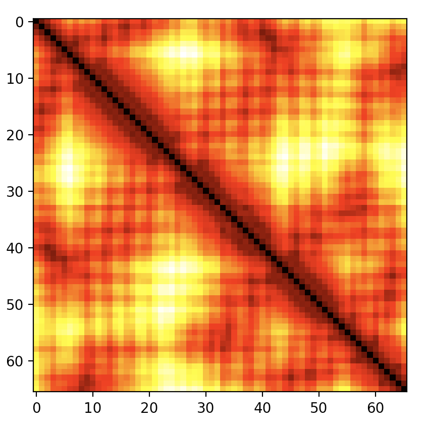
Fig. 4 C-alpha distance plot for PDB file 1A8O (HIV capsid C-terminal domain)
Building a structure from a distance plot
The all-atom distance plot is another representation of a protein structure, also invariant to translation and rotation but lacking in chirality information (a mirror-image structure will generate the same distance plot). By combining the distance matrix with the signs of each dihedral angle, it is possible to regenerate the internal coordinates.
This work uses equations developed by Blue, the Hedronometer, discussed in https://math.stackexchange.com/a/49340/409 and further in http://daylateanddollarshort.com/mathdocs/Heron-like-Results-for-Tetrahedral-Volume.pdf.
To begin, we extract the distances and chirality values from ‘myChain’:
>>> ## create the all-atom distance plot
>>> distances = myCic.distance_plot()
>>> ## get the signs of the dihedral angles
>>> chirality = myCic.dihedral_signs()
We need a valid data structure matching ‘myChain’ to correctly rebuild
it; using read_PIC_seq:math:`` above would work in the general
case, but the 1A8O example used here has some ALTLOC complexity which
the sequence alone would not generate. For demonstration the easiest
approach is to simply duplicate the ‘myChain’ structure, but we set all
the atom and internal coordinate chain arrays to 0s (only for
demonstration) just to be certain there is no data coming through from
the original structure:
>>> ## get new, empty data structure : copy data structure from myChain
>>> myChain2 = IC_duplicate(myChain)[0]["A"]
>>> cic2 = myChain2.internal_coord

>>> ## clear the new atomArray and di/hedra value arrays, just for proof
>>> cic2.atomArray = np.zeros((cic2.AAsiz, 4), dtype=np.float64)
>>> cic2.dihedraAngle[:] = 0.0
>>> cic2.hedraAngle[:] = 0.0
>>> cic2.hedraL12[:] = 0.0
>>> cic2.hedraL23[:] = 0.0
The approach is to regenerate the internal coordinates from the distance plot data, then generate the atom coordinates from the internal coordinates as shown above. To place the final generated structure in the same coordinate space as the starting structure, we copy just the coordinates for the first three N-C\(\alpha\)-C atoms from the chain start of ‘myChain’ to the ‘myChain2’ structure (this is only needed to demonstrate equivalence at end):
>>> ## copy just the first N-Ca-C coords so structures will superimpose:
>>> cic2.copy_initNCaCs(myChain.internal_coord)
The distance_to_internal_coordinates:math:`` routine needs arrays
of the six inter-atom distances for each dihedron for the target
structure. The convenience routine distplot_to_dh_arrays:math:``
extracts these values from the previously generated distance matrix as
needed, and may be replaced by a user method to write these data to the
arrays in the Chain.internal_coords object.
>>> ## copy distances to chain arrays:
>>> cic2.distplot_to_dh_arrays(distances, chirality)
>>> ## compute angles and dihedral angles from distances:
>>> cic2.distance_to_internal_coordinates()
The steps below generate the atom coordinates from the newly generated
‘myChain2’ internal coordinates, then use the Numpy
allclose:math:`` routine to confirm that all values match to
better than PDB file resolution:
>>> ## generate XYZ coordinates from internal coordinates:
>>> myChain2.internal_to_atom_coordinates()
>>> ## confirm result atomArray matches original structure:
>>> np.allclose(cic2.atomArray, myCic.atomArray)
True
Note that this procedure does not use the entire distance matrix, but only the six local distances between the four atoms of each dihedral angle.
Superimposing residues and their neighborhoods
The internal_coords module relies on transforming atom coordinates
between different coordinate spaces for both calculation of torsion
angles and reconstruction of structures. Each dihedron has a coordinate
space transform placing its first atom on the XZ plane, second atom at
the origin, and third atom on the +Z axis, as well as a corresponding
reverse transform which will return it to the coordinates in the
original structure. These transform matrices are available to use as
shown below. By judicious choice of a reference dihedron, pairwise and
higher order residue intereactions can be investigated and visualized
across multiple protein structures, e.g. Fig. 5.
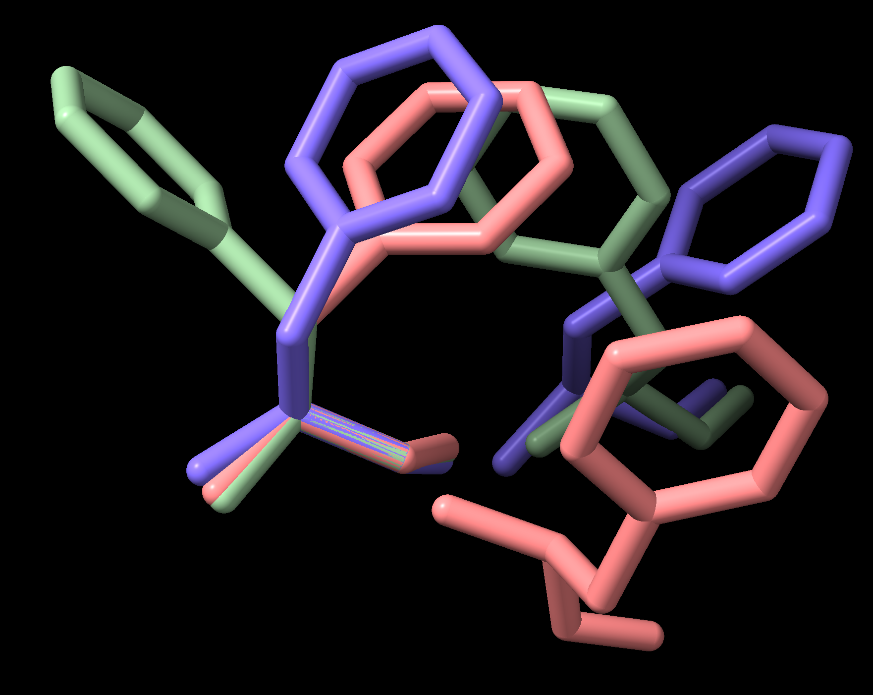
Fig. 5 Neighboring phenylalanine sidechains in PDB file 3PBL (human dopamine D3 receptor)
This example superimposes each PHE residue in a chain on its N-C\(\alpha\)-C\(\beta\) atoms, and presents all PHEs in the chain in the respective coordinate space as a simple demonstration. A more realistic exploration of pairwise sidechain interactions would examine a dataset of structures and filter for interaction classes as discussed in the relevant literature.
# superimpose all phe-phe pairs - quick hack just to demonstrate concept
# for analyzing pairwise residue interactions.  Generates PDB ATOM records
# placing each PHE at origin and showing all other PHEs in environment

## shorthand for key variables:
cic = myChain.internal_coord
resNameNdx = AtomKey.fields.resname
aaNdx = cic.atomArrayIndex

## select just PHE atoms:
pheAtomSelect = [aaNdx.get(k) for k in aaNdx.keys() if k.akl[resNameNdx] == "F"]
aaF = cic.atomArray[pheAtomSelect]  # numpy fancy indexing makes COPY not view

for ric in cic.ordered_aa_ic_list:  # internal_coords version of get_residues()
    if ric.lc == "F":  # if PHE, get transform matrices for chi1 dihedral
        chi1 = ric.pick_angle("chi1")  # N:CA:CB:CG space has C-alpha at origin
        cst = np.transpose(chi1.cst)  # transform TO chi1 space
        # rcst = np.transpose(chi1.rcst)  # transform FROM chi1 space (not needed here)
        cic.atomArray[pheAtomSelect] = aaF.dot(cst)  # transform just the PHEs
        for res in myChain.get_residues():  # print PHEs in new coordinate space
            if res.resname in ["PHE"]:
                print(res.internal_coord.pdb_residue_string())
        cic.atomArray[pheAtomSelect] = aaF  # restore coordinate space from copy
3D printing protein structures
OpenSCAD (https://openscad.org) is a language for creating solid 3D CAD objects. The algorithm to construct a protein structure from internal coordinates is supplied in OpenSCAD with data describing a structure, such that a model can be generated suitable for 3D printing. While other software can generate STL data as a rendering option for 3D printing (e.g. Chimera, https://www.cgl.ucsf.edu/chimera/), this approach generates spheres and cylinders as output and is therefore more amenable to modifications relevant to 3D printing protein structures. Individual residues and bonds can be selected in the OpenSCAD code for special handling, such as highlighting by size or adding rotatable bonds in specific positions (see https://www.thingiverse.com/thing:3957471 for an example).
# write OpenSCAD program of spheres and cylinders to 3d print myChain backbone
## set atom load filter to accept backbone only:
IC_Residue.accept_atoms = IC_Residue.accept_backbone
## set chain break cutoff very high to bridge missing residues with long bonds
IC_Chain.MaxPeptideBond = 4.0
## delete existing data to force re-read of all atoms with attributes set above:
myChain.internal_coord = None
write_SCAD(myChain, "myChain.scad", scale=10.0)
internal_coords control attributes
A few control attributes are available in the internal_coords
classes to modify or filter data as internal coordinates are calculated.
These are listed in Table Control attributes in Bio.PDB.internal_coords.:
Class |
Attribute |
Default |
Effect |
|---|---|---|---|
AtomKey |
d2h |
False |
Convert D atoms to H if True |
IC_Chain |
MaxPeptideBond |
1.4 |
Max C-N length w/o chain break; make large to link over missing residues for 3D models |
IC_Residue |
accept_atoms |
mainchain, hydrogen atoms |
override to remove some or all sidechains, H’s, D’s |
IC_Residue |
accept_resnames |
CYG, YCM, UNK |
3-letter names for HETATMs to process, backbone only unless added to ic_data.py |
IC_Residue |
gly_Cbeta |
False |
override to generate Gly C\(\beta\) atoms based on database averages |
Determining atom-atom contacts
Use NeighborSearch to perform neighbor lookup. The neighbor lookup
is done using a KD tree module written in C (see the KDTree class in
module Bio.PDB.kdtrees), making it very fast. It also includes a
fast method to find all point pairs within a certain distance of each
other.
Calculating the Half Sphere Exposure
Half Sphere Exposure (HSE) is a new, 2D measure of solvent exposure [Hamelryck2005]. Basically, it counts the number of C\(\alpha\) atoms around a residue in the direction of its side chain, and in the opposite direction (within a radius of 13 Å. Despite its simplicity, it outperforms many other measures of solvent exposure.
HSE comes in two flavors: HSE\(\alpha\) and HSE\(\beta\).
The former only uses the C\(\alpha\) atom positions, while the
latter uses the C\(\alpha\) and C\(\beta\) atom positions.
The HSE measure is calculated by the HSExposure class, which can
also calculate the contact number. The latter class has methods which
return dictionaries that map a Residue object to its corresponding
HSE\(\alpha\), HSE\(\beta\) and contact number values.
Example:
>>> model = structure[0]
>>> hse = HSExposure()
# Calculate HSEalpha
>>> exp_ca = hse.calc_hs_exposure(model, option="CA3")
# Calculate HSEbeta
>>> exp_cb = hse.calc_hs_exposure(model, option="CB")
# Calculate classical coordination number
>>> exp_fs = hse.calc_fs_exposure(model)
# Print HSEalpha for a residue
>>> print(exp_ca[some_residue])
Determining the secondary structure
For this functionality, you need to install DSSP (and obtain a license
for it — free for academic use, see
https://swift.cmbi.umcn.nl/gv/dssp/). Then use the DSSP class, which
maps Residue objects to their secondary structure (and accessible
surface area). The DSSP codes are listed in
Table DSSP codes in Bio.PDB.. Note that DSSP (the program, and thus
by consequence the class) cannot handle multiple models!
Code |
Secondary structure |
|---|---|
H |
\(\alpha\)-helix |
B |
Isolated \(\beta\)-bridge residue |
E |
Strand |
G |
3-10 helix |
I |
\(\Pi\)-helix |
T |
Turn |
S |
Bend |
Other |
The DSSP class can also be used to calculate the accessible surface
area of a residue. But see also section Calculating the residue depth.
Calculating the residue depth
Residue depth is the average distance of a residue’s atoms from the
solvent accessible surface. It’s a fairly new and very powerful
parameterization of solvent accessibility. For this functionality, you
need to install Michel Sanner’s MSMS program
(https://www.scripps.edu/sanner/html/msms_home.html). Then use the
ResidueDepth class. This class behaves as a dictionary which maps
Residue objects to corresponding (residue depth, C\(\alpha\)
depth) tuples. The C\(\alpha\) depth is the distance of a
residue’s C\(\alpha\) atom to the solvent accessible surface.
Example:
>>> model = structure[0]
>>> rd = ResidueDepth(model, pdb_file)
>>> residue_depth, ca_depth = rd[some_residue]
You can also get access to the molecular surface itself (via the
get_surface function), in the form of a Numeric Python array with
the surface points.
Superimposing two structures
Superimposing identical sets of atoms
Use a Superimposer object to superimpose two coordinate sets. This
object calculates the rotation and translation matrix that rotates two
lists of atoms on top of each other in such a way that their RMSD is
minimized. Of course, the two lists need to contain the same number of
atoms. The Superimposer object can also apply the
rotation/translation to a list of atoms. The rotation and translation
are stored as a tuple in the rotran attribute of the
Superimposer object (note that the rotation is right multiplying!).
The RMSD is stored in the rms attribute.
To reiterate, the Superimposer object requires two lists of atoms
that must contain an identical number. To align two chains with similar
but not identical sequences, use the CEAligner (described below)
The algorithm used by Superimposer comes from
Golub & Van Loan [Golub1989] and makes use of
singular value decomposition (this is implemented in the general
Bio.SVDSuperimposer module).
Example:
>>> from Bio.PDB import Superimposer
>>> sup = Superimposer()
# Specify the atom lists
# 'fixed' and 'moving' are lists of Atom objects
# The moving atoms will be put on the fixed atoms
>>> sup.set_atoms(fixed, moving)
# Print rotation/translation/rmsd
>>> print(sup.rotran)
>>> print(sup.rms)
# Apply rotation/translation to the moving atoms
>>> sup.apply(moving)
To superimpose two structures based on their active sites, use the active site atoms to calculate the rotation/translation matrices (as above), and apply these to the whole molecule.
In addition to using the Superimposer object, you can also choose
to use the QCPSuperimposer object, which is faster than the
standard Superimposer.
The algorithm for the QCPSuperimposer comes from Theobald [Theobald2005]
and rapidly calculates the minimum RMSD by using the quaternion characteristic
polynomial (QCP).
The implementation is very similar to the Superimposer
>>> from Bio.PDB.qcprot import QCPSuperimposer
>>> sup = QCPSuperimposer()
# Specify the atom lists
# 'fixed' and 'moving' are lists of Atom objects
# The moving atoms will be put on the fixed atoms
>>> sup.set_atoms(fixed, moving)
# Print rotation/translation/rmsd
>>> print(sup.rotran)
>>> print(sup.rms)
# Apply rotation/translation to the moving atoms
>>> sup.apply(moving)
Aligning dissimilar structures
If you want to align two structures with low sequence identity (less than 50%)
you can use the CEAligner class, which implements the Combinatorial Extension (CE)
algorithm for structural alignment. This method automatically finds the best matching
regions between two structures and superimposes them by using the C-alpha coordinates
(for proteins) or C4’ (for nucleic acids)
The algorithm used in the CEAligner class is from Shindyalov & Bourne [Shindyalov1998]
and uses the QCPSuperimposer to perform the actual superimposition after discovering
the best matching regions
Example:
>>> from Bio.PDB.cealign import CEAligner
>>> aligner = CEAligner()
>>> aligner.set_reference(structure1)
>>> aligner.align(structure2)
# Get RMSD of the best alignment
>>> print(aligner.rms)
This is useful for comparing proteins with significantly different sequences. By default,
the align function will apply the transformation to structure2 as well as calculate the
RMSD. To just calculate optimal RMSD without changing the structure2 coordinates, pass
transform=False.
Common problems in PDB files
It is well known that many PDB files contain semantic errors (not the structures themselves, but their representation in PDB files). Bio.PDB tries to handle this in two ways. The PDBParser object can behave in two ways: a restrictive way and a permissive way, which is the default.
Example:
# Permissive parser
>>> parser = PDBParser(PERMISSIVE=1)
>>> parser = PDBParser()  # The same (default)
# Strict parser
>>> strict_parser = PDBParser(PERMISSIVE=0)
In the permissive state (DEFAULT), PDB files that obviously contain errors are “corrected” (i.e. some residues or atoms are left out). These errors include:
Multiple residues with the same identifier
Multiple atoms with the same identifier (taking into account the altloc identifier)
These errors indicate real problems in the PDB file (for details see Hamelryck and Manderick, 2003 [Hamelryck2003A]). In the restrictive state, PDB files with errors cause an exception to occur. This is useful to find errors in PDB files.
Some errors however are automatically corrected. Normally each disordered atom should have a non-blank altloc identifier. However, there are many structures that do not follow this convention, and have a blank and a non-blank identifier for two disordered positions of the same atom. This is automatically interpreted in the right way.
Sometimes a structure contains a list of residues belonging to chain A, followed by residues belonging to chain B, and again followed by residues belonging to chain A, i.e. the chains are ’broken’. This is also correctly interpreted.
Examples
The PDBParser/Structure class was tested on about 800 structures (each belonging to a unique SCOP superfamily). This takes about 20 minutes, or on average 1.5 seconds per structure. Parsing the structure of the large ribosomal subunit (1FKK), which contains about 64000 atoms, takes 10 seconds on a 1000 MHz PC.
Three exceptions were generated in cases where an unambiguous data structure could not be built. In all three cases, the likely cause is an error in the PDB file that should be corrected. Generating an exception in these cases is much better than running the chance of incorrectly describing the structure in a data structure.
Duplicate residues
One structure contains two amino acid residues in one chain with the same sequence identifier (resseq 3) and icode. Upon inspection it was found that this chain contains the residues Thr A3, …, Gly A202, Leu A3, Glu A204. Clearly, Leu A3 should be Leu A203. A couple of similar situations exist for structure 1FFK (which e.g. contains Gly B64, Met B65, Glu B65, Thr B67, i.e. residue Glu B65 should be Glu B66).
Duplicate atoms
Structure 1EJG contains a Ser/Pro point mutation in chain A at position 22. In turn, Ser 22 contains some disordered atoms. As expected, all atoms belonging to Ser 22 have a non-blank altloc specifier (B or C). All atoms of Pro 22 have altloc A, except the N atom which has a blank altloc. This generates an exception, because all atoms belonging to two residues at a point mutation should have non-blank altloc. It turns out that this atom is probably shared by Ser and Pro 22, as Ser 22 misses the N atom. Again, this points to a problem in the file: the N atom should be present in both the Ser and the Pro residue, in both cases associated with a suitable altloc identifier.
Automatic correction
Some errors are quite common and can be easily corrected without much risk of making a wrong interpretation. These cases are listed below.
A blank altloc for a disordered atom
Normally each disordered atom should have a non-blank altloc identifier. However, there are many structures that do not follow this convention, and have a blank and a non-blank identifier for two disordered positions of the same atom. This is automatically interpreted in the right way.
Broken chains
Sometimes a structure contains a list of residues belonging to chain A, followed by residues belonging to chain B, and again followed by residues belonging to chain A, i.e. the chains are “broken”. This is correctly interpreted.
Fatal errors
Sometimes a PDB file cannot be unambiguously interpreted. Rather than guessing and risking a mistake, an exception is generated, and the user is expected to correct the PDB file. These cases are listed below.
Duplicate residues
All residues in a chain should have a unique id. This id is generated based on:
The sequence identifier (resseq).
The insertion code (icode).
The hetfield string (“W” for waters and “H_” followed by the residue name for other hetero residues)
The residue names of the residues in the case of point mutations (to store the Residue objects in a DisorderedResidue object).
If this does not lead to a unique id something is quite likely wrong, and an exception is generated.
Duplicate atoms
All atoms in a residue should have a unique id. This id is generated based on:
The atom name (without spaces, or with spaces if a problem arises).
The altloc specifier.
If this does not lead to a unique id something is quite likely wrong, and an exception is generated.
Accessing the Protein Data Bank
Downloading structures from the Protein Data Bank
Structures can be downloaded from the PDB (Protein Data Bank) by using
the retrieve_pdb_file method on a PDBList object. The argument
for this method is the PDB identifier of the structure.
>>> pdbl = PDBList()
>>> pdbl.retrieve_pdb_file("1FAT")
The PDBList class can also be used as a command-line tool:
python PDBList.py 1fat
The downloaded file will be called pdb1fat.ent and stored in the
current working directory. Note that the retrieve_pdb_file method
also has an optional argument pdir that specifies a specific
directory in which to store the downloaded PDB files.
The retrieve_pdb_file method also has some options to specify the
compression format used for the download, and the program used for local
decompression (default .Z format and gunzip). In addition, the
PDB ftp site can be specified upon creation of the PDBList object.
By default, the server of the Worldwide Protein Data Bank
(ftp://ftp.wwpdb.org/pub/pdb/data/structures/divided/pdb/) is used. See
the API documentation for more details. Thanks again to Kristian Rother
for donating this module.
Downloading the entire PDB
The following commands will store all PDB files in the /data/pdb
directory:
python PDBList.py all /data/pdb

python PDBList.py all /data/pdb -d
The API method for this is called download_entire_pdb. Adding the
-d option will store all files in the same directory. Otherwise,
they are sorted into PDB-style subdirectories according to their PDB
ID’s. Depending on the traffic, a complete download will take 2-4 days.
Keeping a local copy of the PDB up to date
This can also be done using the PDBList object. One simply creates a
PDBList object (specifying the directory where the local copy of the
PDB is present) and calls the update_pdb method:
>>> pl = PDBList(pdb="/data/pdb")
>>> pl.update_pdb()
One can of course make a weekly cronjob out of this to keep the
local copy automatically up-to-date. The PDB ftp site can also be
specified (see API documentation).
PDBList has some additional methods that can be of use. The
get_all_obsolete method can be used to get a list of all obsolete
PDB entries. The changed_this_week method can be used to obtain the
entries that were added, modified or obsoleted during the current week.
For more info on the possibilities of PDBList, see the API
documentation.
General questions
How well tested is Bio.PDB?
Pretty well, actually. Bio.PDB has been extensively tested on nearly 5500 structures from the PDB - all structures seemed to be parsed correctly. More details can be found in the Bio.PDB Bioinformatics article. Bio.PDB has been used/is being used in many research projects as a reliable tool. In fact, I’m using Bio.PDB almost daily for research purposes and continue working on improving it and adding new features.
How fast is it?
The PDBParser performance was tested on about 800 structures (each
belonging to a unique SCOP superfamily). This takes about 20 minutes, or
on average 1.5 seconds per structure. Parsing the structure of the large
ribosomal subunit (1FKK), which contains about 64000 atoms, takes 10
seconds on a 1000 MHz PC. In short: it’s more than fast enough for many
applications.
Is there support for molecular graphics?
Not directly, mostly since there are quite a few Python based/Python aware solutions already, that can potentially be used with Bio.PDB. My choice is Pymol, BTW (I’ve used this successfully with Bio.PDB, and there will probably be specific PyMol modules in Bio.PDB soon/some day). Python based/aware molecular graphics solutions include:
PyMol: https://pymol.org/
Chimera: https://www.cgl.ucsf.edu/chimera/
CCP4mg: http://www.ccp4.ac.uk/MG/
Who’s using Bio.PDB?
Bio.PDB was used in the construction of DISEMBL, a web server that predicts disordered regions in proteins (http://dis.embl.de/). Bio.PDB has also been used to perform a large scale search for active sites similarities between protein structures in the PDB [Hamelryck2003B], and to develop a new algorithm that identifies linear secondary structure elements [Majumdar2005].
Judging from requests for features and information, Bio.PDB is also used by several LPCs (Large Pharmaceutical Companies :-).